Identifying Bias in Spatial Scales Using Statistical Analysis
Author
Sojung Chu
Published
December 18, 2025
Master Splinter
Introduction
This report is my individual component of a group final course project with Shreya, Rachel, Geraldine, David, and Wing. Initially, we wanted to solve the case of the pesky rats that rule over New York City (NYC) by finding a correlation between the 311 rodent complaints, which are often used as markers for where the rats are located, and other factors. While much of the existing research focuses on identifying the factors that lead to rat infestations, our study instead examined whether 311 rodent complaints are an accurate proxy for rat prevalence. We investigated whether reliance on 311 data introduces bias.
Specific Research Question: Does spatial aggregation cause 311 rodent calls to reflect reporting behavior rather than rat activity?
My analysis addresses whether spatial aggregation causes rodent complaints to reflect reporting behavior rather than rat activity. In 2017, NYC began designating Rat Mitigation Zones, with one criterion being the number of rat-related 311 complaints at the community district level. A difference-in-differences approach was used to compare 311 rodent complaints before and after a rodent inspection, with a passed inspection treated as the event at time zero. With inferring that a passed inspection signals acceptable rat conditions, we expect complaints to decline within the spatial unit after a passed inspection, provided the unit accurately captures rodent activity. This expectation was evaluated at three spatial scales: a local 150‑meter radius, Neighborhood Tabulation Areas (NTA) to maintain consistency with my groupmate’s analysis, and Community Districts to align with how NYC aggregates 311 rat complaints.
The technical details of the analysis, including data acquisition, data cleaning, exploratory data analysis, and model estimation, are documented in this report. Reproducible code and detailed explanations illustrating how difference-in-differences models were developed and evaluated using NYC data are also included. All analyses were conducted in R through associated packages.
Methodology
The following methods were used to obtain and reconstruction four datasets to prepare for analysis.
Data Acquisition
Data was downloaded responsibly through functions that only download the required data if it does not already exist. Before this, the process starts by loading necessary packages through a helper function that installs and loads R packages used throughout this report.
Code
#' Install and load an R package if it is not already available.#'#' @param pkg A character string specifying the name of the package to load.#' @return Invisibly returns TRUE if the package is successfully loaded.#' @examples#' load_package("tidyr")load_package <-function(pkg) {if (!requireNamespace(pkg, quietly =TRUE)) {install.packages(pkg) }suppressPackageStartupMessages(library(pkg, character.only =TRUE))}PACKAGES <-c("httr2", "jsonlite", "dplyr", "sf", "purrr", "tidyr", "broom","lubridate", "readr", "tidyverse", "nngeo", "ggplot2", "fixest", "nngeo", "scales","knitr", "ggrepel", "kableExtra", "shiny", "leaflet", "data.table", "modelsummary").loaded <-lapply(PACKAGES, load_package)
Rodent Inspections
The NYC Rat Inspection dataset contains records of rodent inspections conducted across the five boroughs in response to public complaints and routine monitoring. This dataset is compiled and published by the New York City Department of Health and Mental Hygiene (DOHMH) and is publicly available through NYC Open Data. The dataset contains approximately 2.9 million records, with a small number of inspections dated between 1918 and 1971 and two records from 2000, but these early outliers were removed. The majority of observations begin on January 1, 2001, and extend through December 8, 2025. Each record represents an individual inspection and includes information such as the inspection date, inspection outcome, and location details. Some records list inspection dates in 2045. These future-dated entries were identified as data errors and were removed.
Code
#' Download and cache NYC rat inspection records from NYC Open Data.#'#' This chunk defines a helper function that retrieves rat inspection records from the#' NYC Open Data API and stores a local cached copy for reuse in future runs. Because#' the dataset can exceed single-request limits, the function downloads the data in#' paginated batches using `$limit` and `$offset`, combines the batches into a single#' table, and saves the result as a CSV in the project data directory. If a cached file#' already exists and `refresh = FALSE`, the function reads the local CSV instead of#' re-downloading the data.#'#' @return A tibble containing the full set of rat inspection records returned by the#' NYC Open Data endpoint.#' @examples#' rat_inspection <- load_rat_inspection()# Ensure a local directory exists for storing cached API downloads.# Caching downloaded files allows the analysis to be rerun without# repeatedly querying the NYC Open Data API.if (!dir.exists("data/final")) {dir.create("data/final", showWarnings =FALSE, recursive =TRUE)}load_rat_inspection <-function(refresh =FALSE) {# Define a local cache path so the dataset can be reused across runs.# Caching avoids repeated API calls and makes the workflow reproducible. target_dir <-"data/final" f_name <-"rat_inspection.csv" file_path <-file.path(target_dir, f_name)# Create the cache directory if it does not already exist.if (!dir.exists(target_dir)) {dir.create(target_dir, recursive =TRUE) }# If no cached file is available, or if a refresh is requested, download the data.# Otherwise, read the previously saved file from disk.if (!file.exists(file_path) || refresh) {message("Downloading full rat inspection dataset from NYC Open Data...")# Specify the NYC Open Data endpoint used to retrieve the inspection records. base_url <-"https://data.cityofnewyork.us/resource/p937-wjvj.json"# The Socrata API limits the number of rows returned per request, so the full# dataset is retrieved in repeated chunks using limit and offset parameters. chunk_limit <-50000L all_chunks <-list() offset <-0L chunk_id <-1Lrepeat {message("Requesting rows with offset = ", offset, " ...") resp <-request(base_url) |>req_url_query("$limit"= chunk_limit,"$offset"= offset ) |>req_perform()# Stop execution if the API request fails.resp_check_status(resp)# Parse the response into a tabular object that can be combined across chunks.# Flattening is used to bring nested fields into regular columns when present. raw_json <-resp_body_string(resp) dat_list <-fromJSON(raw_json, flatten =TRUE) chunk_tbl <- dat_list |>as_tibble() n_chunk <-nrow(chunk_tbl)message("Retrieved ", n_chunk, " rows in chunk ", chunk_id, ".")# A zero-row response indicates the end of the export.if (n_chunk ==0) {message("No more rows returned. Reached end of dataset.")break } all_chunks[[chunk_id]] <- chunk_tbl# If the chunk is smaller than the request limit, assume this is the final page.if (n_chunk < chunk_limit) {message("Final chunk returned fewer than ", chunk_limit, " rows.")break }# Otherwise, advance the offset and request the next batch. offset <- offset + n_chunk chunk_id <- chunk_id +1L }# Combine all retrieved chunks into a single table. rat_inspection <-bind_rows(all_chunks)message("Total rows downloaded: ", nrow(rat_inspection))# Save the assembled dataset so it can load it from disk.write_csv(rat_inspection, file_path) } else {message("Reading existing rat inspection data from CSV...") rat_inspection <-read_csv(file_path, show_col_types =FALSE) } rat_inspection}rat_inspection <-load_rat_inspection()# Filter out inspection records with implausible dates that likely reflect data issues.# This removes a small number of records dated 1918–1971, the two records from 2000,# and outliers dated in 2045.rat_inspection <- rat_inspection |>mutate(inspection_date =as_date(inspection_date)) |>filter(!is.na(inspection_date)) |>filter(year(inspection_date) >=1972,year(inspection_date) <=2024) |>filter(year(inspection_date) !=2000)
311 Rodent Complaints
The New York City 311 Rodent Complaints data set contains records of service requests submitted by residents reporting rodent sightings. This dataset is compiled and made publicly available through the NYC Open Data portal and from the NYC 311 service system. It contains approximately 492,000 records and spans from January 2010 through December 2025. Each record includes information such as the date the complaint was submitted, complaint type, and location details.
Code
#' Download and assemble NYC 311 rodent complaint records from NYC Open Data.#'#' This chunk prepares a local data directory and defines a helper function that#' retrieves NYC 311 rodent complaint data from the NYC Open Data API. Because the#' dataset can exceed single-request limits, the function downloads the data in#' paginated batches using `$limit` and `$offset`. Each batch is cached locally as#' a GeoJSON file to avoid repeated downloads and to make the workflow reproducible.#' The cached batches are then read with `st_read()` and combined into a single dataset.#'#' @return An `sf` object containing the full set of rodent complaint records returned#' by the NYC Open Data endpoint.#' @examples#' rodent_complaints <- get_rodent_complaints()# Define a helper function to download and assemble NYC 311 rodent complaint data.# The function retrieves the data in batches to accommodate API request limits,# caches each batch locally as a GeoJSON file, and combines all batches into# a single sf object for downstream analysis.get_rodent_complaints <-function() {# Define the NYC Open Data API endpoint for 311 rodent complaints.# The data are served as GeoJSON and must be retrieved in multiple requests. ENDPOINT <-"https://data.cityofnewyork.us/resource/cvf2-zn8s.geojson" BATCH_SIZE <-50000 OFFSET <-0 END_OF_EXPORT <-FALSE FILE_INDEX <-1 ALL_DATA <-list()# Continue requesting data until the API returns fewer rows than the batch size,# which signals that the end of the dataset has been reached.while (!END_OF_EXPORT) {# Construct a stable filename for the current batch so that it can be reused# across multiple runs of the analysis. file_name <-sprintf("rodent_311_%04d.geojson", FILE_INDEX) file_path <-file.path("data/final", file_name)# Download the current batch only if it has not already been saved locally.# This avoids unnecessary API calls and improves reproducibility.if (!file.exists(file_path)) { req <-request(ENDPOINT) |>req_url_query(`$limit`= BATCH_SIZE,`$offset`= OFFSET ) resp <-req_perform(req)resp_check_status(resp)resp_body_raw(resp) |>writeBin(con = file_path) }# Read the cached GeoJSON batch into an sf object. batch_data <-st_read(file_path, quiet =TRUE)# Append the current batch to the list of all downloaded data. ALL_DATA <-c(ALL_DATA, list(batch_data))# If the number of returned rows is smaller than the requested batch size,# the final page has been reached and the loop can terminate.if (NROW(batch_data) != BATCH_SIZE) { END_OF_EXPORT <-TRUE } else { OFFSET <- OFFSET + BATCH_SIZE FILE_INDEX <- FILE_INDEX +1 } }# Combine all downloaded batches into a single sf object. ALL_DATA <-bind_rows(ALL_DATA)return(ALL_DATA)}# Execute the data download and combination step and store the result.rodent_complaints <-get_rodent_complaints()
Neighborhood Tabulation Areas (NTA)
The 2020 New York City Neighborhood Tabulation Area (NTA) boundary polygons were downloaded from an ArcGIS REST service provided by the City of New York. These polygons define standardized neighborhood units commonly used for demographic and public health analyses. The boundary file was cached locally to ensure reproducibility and loaded as a spatial object, then transformed to align with the rodent inspection and 311 complaint data.
Code
#' Download and load NYC Neighborhood Tabulation Area (NTA) boundary polygons.#'#' This function downloads the 2020 Neighborhood Tabulation Area boundary polygons from an#' ArcGIS REST endpoint and caches the GeoJSON locally for reuse. If the file already exists#' locally, it is read from disk instead of being downloaded again.#' The boundaries are loaded as an `sf` object and transformed to EPSG:4326 to align with#' the coordinate reference system used by the rodent datasets.#'#' @param nta_url URL of the ArcGIS GeoJSON endpoint (default provided).#' @param nta_path Local filepath used to cache the downloaded GeoJSON.#' @return An `sf` object containing NYC Neighborhood Tabulation Area polygon geometries#' and associated attributes.#' @importFrom httr2 request req_perform resp_check_status resp_body_raw#' @importFrom sf st_read st_transform#' @exportload_nta_boundaries <-function(nta_url ="https://services5.arcgis.com/GfwWNkhOj9bNBqoJ/arcgis/rest/services/NYC_Neighborhood_Tabulation_Areas_2020/FeatureServer/0/query?where=1=1&outFields=*&outSR=4326&f=pgeojson",nta_path ="data/final/nta_2020.geojson",refresh =FALSE) {# Ensure the output directory exists before attempting to write cached files. out_dir <-dirname(nta_path)if (!dir.exists(out_dir)) {dir.create(out_dir, recursive =TRUE) }# Download the file only if it is not already cached locally.# This keeps the workflow reproducible and avoids repeated requests to the server.if (!file.exists(nta_path)) { resp <-request(nta_url) |>req_perform()resp_check_status(resp)resp_body_raw(resp) |>writeBin(con = nta_path) }# Read the cached NTA boundaries as an sf object and standardize the CRS.# Using a consistent CRS ensures spatial joins and distance calculations work as expected. nta <-st_read(nta_path, quiet =TRUE) |>st_transform(4326)return(nta)}nta <-load_nta_boundaries()
Community Districts
The New York City Community District boundary polygons were downloaded from the NYC Department of City Planning’s dataset, using an ArcGIS REST endpoint that provides the boundaries in GeoJSON format. The boundary file was also cached locally.
Code
#' Download and load NYC Community District boundary polygons.#'#' This function downloads NYC Department of City Planning Community District boundaries#' from an ArcGIS REST endpoint and caches the GeoJSON locally for reuse. If the file#' already exists locally, it is read from disk instead of being downloaded again. #' The boundaries are loaded as an `sf` object and transformed to to ensure compatibility#' with other datasets used in the analysis.#'#' @param cd_url URL of the ArcGIS GeoJSON endpoint (default provided).#' @param cd_path Local filepath used to cache the downloaded GeoJSON#' (default "data/final/community_districts.geojson").#' @return An `sf` object containing Community District polygons. The returned object#' includes the Community District identifier (`BoroCD`) and geometry.#' @importFrom httr2 request req_perform resp_check_status resp_body_raw#' @importFrom sf st_read st_transform#' @importFrom dplyr select#' @exportload_cd_shapefiles <-function(cd_url ="https://services5.arcgis.com/GfwWNkhOj9bNBqoJ/arcgis/rest/services/NYC_Community_Districts/FeatureServer/0/query?where=1=1&outFields=*&outSR=4326&f=pgeojson",cd_path ="data/final/community_districts.geojson",refresh =FALSE) {# Ensure the output directory exists before attempting to write cached files. out_dir <-dirname(cd_path)if (!dir.exists(out_dir)) {dir.create(out_dir, recursive =TRUE) }# Download the GeoJSON only when needed to minimize repeated server requests.if (refresh ||!file.exists(cd_path)) { resp <-request(cd_url) |>req_perform()resp_check_status(resp)resp_body_raw(resp) |>writeBin(con = cd_path) }# Read the cached GeoJSON and standardize to EPSG:4326 for spatial compatibility. cd <-st_read(cd_path, quiet =TRUE) |>st_transform(4326)# Keep only the Community District identifier and geometry used for joins. cd <- cd |>select(BoroCD, geometry)return(cd)}cd_keep <-load_cd_shapefiles()
Data Integration
Since the rodent inspection and 311 complaint data are recorded at the point level using latitude and longitude coordinates, I standardized the geographic unit of analysis across the 311 rodent complaint and rodent inspection datasets. Point locations were converted to spatial features and spatially joined to 2020 NTA boundary polygons using a point-in-polygon approach, assigning each record to an NTA.
Code
# Convert rodent complaint coordinates into sf point features.# Extract longitude and latitude as numeric values and remove records without valid coordinates.rat_coords <- rodent_complaints |>mutate(lon =as.numeric(longitude),lat =as.numeric(latitude) ) |>drop_na(lon, lat)# Convert the complaint records into an sf object so spatial operations can be applied.rats_sf <-st_as_sf( rat_coords,coords =c("lon", "lat"),crs =4326)# Load the NTA polygon boundaries and make sure they are in the same CRS as the complaint points.nta <-st_read("data/final/nta_2020.geojson", quiet =TRUE) |>st_transform(4326)# Create a lookup table mapping NTA names to official NTA codes for later joins.nta_lookup <- nta |>st_drop_geometry() |>select(nta = NTAName, nta_code = NTA2020 ) |>distinct()# Spatial join NTA attributes onto each complaint point.rat311_with_nta <-st_join( rats_sf, nta[, c("NTA2020", "NTAName", "BoroName")])# Drop geometry to work with a regular tabular data frame while keeping the NTA attributes.rat311_with_nta_df <- rat311_with_nta |>st_drop_geometry()
Community district polygons were then joined in a similar way.
Code
# Spatial join: assign each 311 rat point to a Community District (BoroCD)rat311_with_cd <-st_join(rats_sf, cd_keep)# Drop geometry for a regular tibblerat311_with_cd_df <- rat311_with_cd |>st_drop_geometry()# Drop geometry for a regular tabular data framerat311_with_cd_df <- rat311_with_cd |>st_drop_geometry()# Add Community District (BoroCD) to any NYC dataset with lon/lat columns# Keeps pipeline modular: load raw data first, enrich later, without modifying originals.add_cd_to_points <-function(df,lon_col ="longitude",lat_col ="latitude",cd_path ="data/final/community_districts.geojson") {# Read/prepare Community District polygons (lightweight) cd_keep <-st_read(cd_path, quiet =TRUE) |>st_transform(4326) |>select(BoroCD, geometry)# Extract coords + drop missing df_coords <- df |>mutate(lon =as.numeric(.data[[lon_col]]),lat =as.numeric(.data[[lat_col]]) ) |>drop_na(lon, lat)# Convert to sf points df_sf <-st_as_sf(df_coords, coords =c("lon", "lat"), crs =4326)# Spatial join + return as regular tibble (no geometry column)st_join(df_sf, cd_keep, left =TRUE) |>st_drop_geometry()}rat_inspection_with_cd_df <-add_cd_to_points(rat_inspection)rat311_with_cd_df <-add_cd_to_points(rodent_complaints)
Data Construction
In order to implement a event-centered difference-in-differences design, balanced panels were constructed around the timing of passed rodent inspections. For each spatial scale, inspection events were treated as the focal intervention, and 311 rodent complaints were organized relative to the first passed inspection within a given geographic unit. All panels were constructed at the weekly level and retain weeks with zero complaints.
150 Meter Radius
Code
#' Construct distance-based difference-in-differences panels around PASS inspections.#'#' To support the distance-based difference-in-differences analysis, this chunk integrates#' 311 rodent complaint records with PASS inspection locations using a spatial proximity#' approach. Both datasets are converted to spatial point features and projected to a#' coordinate reference system that preserves distances in meters. This allows complaint#' activity to be measured within a fixed radius of each inspection site and enables#' spatial proximity to be incorporated directly into the DiD design.#'#' The resulting data structure supports neighborhood-by-month panels with zero-call#' months included and is used to estimate Poisson DiD models with neighborhood and#' month fixed effects.# Specify the radius, in meters, used to define complaints occurring near a PASS inspection.# This value determines the spatial scale at which inspection effects are evaluated.# -----------------------------# WEEK VERSION (separate names) + recommended filters# -----------------------------radius_m_w <-150window_w_w <-26week_start_w <-1# 1 = Monday, 7 = Sunday# 1) 311 calls -> sf points with weekcalls_sf_w <- rat311_with_nta_df %>%filter(!is.na(longitude), !is.na(latitude)) %>%mutate(created_date_w =as.Date(created_date),call_week_w =floor_date(created_date_w, "week", week_start = week_start_w) ) %>%st_as_sf(coords =c("longitude", "latitude"), crs =4326) %>%st_transform(3857)# 2) Inspections -> sf points with week (PASS centers)insp_sf_w <- rat_inspection %>%filter(!is.na(longitude), !is.na(latitude)) %>%mutate(inspection_date_w =ymd(inspection_date),inspection_week_w =floor_date(inspection_date_w, "week", week_start = week_start_w) ) %>%st_as_sf(coords =c("longitude", "latitude"), crs =4326) %>%st_transform(3857)pass_sf_w <- insp_sf_w %>%filter(result =="Passed") %>%arrange(inspection_week_w) %>%mutate(neigh_id_w =row_number(),first_pass_week_w = inspection_week_w )# 3) Nearest PASS for each call within radiusnn_out_w <-st_nn( calls_sf_w, pass_sf_w,k =1, maxdist = radius_m_w,returnDist =TRUE,progress =FALSE)calls_sf_w <- calls_sf_w %>%mutate(pass_row_w =map_int(nn_out_w$nn, ~if (length(.x) ==0) NA_integer_else .x[1]),dist_to_pass_m_w =map_dbl(nn_out_w$dist, ~if (length(.x) ==0) NA_real_else .x[1]),neigh_id_w =if_else(is.na(pass_row_w), NA_integer_, pass_sf_w$neigh_id_w[pass_row_w]) ) %>%select(-pass_row_w)# 4) Keep only calls within chosen radius of a PASScalls_near_w <- calls_sf_w %>%filter(!is.na(dist_to_pass_m_w) & dist_to_pass_m_w <= radius_m_w)# 5) Aggregate to neighborhood × week: count callscalls_neigh_week_w <- calls_near_w %>%st_drop_geometry() %>%group_by(neigh_id_w, call_week_w) %>%summarise(calls_w =n(), .groups ="drop")# PASS event info per neigh_id_wpass_info_w <- pass_sf_w %>%st_drop_geometry() %>%select(neigh_id_w, first_pass_week_w)# 6) FULL PANEL: all neighborhoods × all weeks (fill zeros) + event-time varsall_weeks_w <-seq(from =min(calls_neigh_week_w$call_week_w, na.rm =TRUE),to =max(calls_neigh_week_w$call_week_w, na.rm =TRUE),by ="week")# Only neighborhoods that actually get used (nearest for >=1 call within radius)all_neigh_w <-sort(unique(calls_near_w$neigh_id_w))full_neigh_panel_w <-expand.grid(neigh_id_w = all_neigh_w,call_week_w = all_weeks_w)panel_neigh_w <- full_neigh_panel_w %>%left_join(calls_neigh_week_w, by =c("neigh_id_w", "call_week_w")) %>%mutate(calls_w =replace_na(calls_w, 0L)) %>%left_join(pass_info_w, by ="neigh_id_w") %>%mutate(rel_week_w =as.integer((call_week_w - first_pass_week_w) /7),post_pass_w =as.integer(rel_week_w >=0) ) %>%filter(rel_week_w >=-window_w_w, rel_week_w <= window_w_w)# 7) Recommended filters (balanced window + drop all-zero centers)panel_neigh_w <- panel_neigh_w %>%group_by(neigh_id_w) %>%mutate(n_pre_w =sum(rel_week_w <0),n_post_w =sum(rel_week_w >=0),total_calls_w =sum(calls_w, na.rm =TRUE) ) %>%ungroup() %>%filter( n_pre_w >=1, n_post_w >=1, total_calls_w >0 ) %>%select(-total_calls_w)
A distance-based neighborhood radius was constructed around each passed inspection to capture localized responses in 311 complaints. A 150-meter radius was selected to reflect the spatial range over which an inspection could influence nearby complaint behavior while minimizing spillovers from unrelated areas. Each complaint was linked to its nearest passed inspection within this radius, creating inspection-centered neighborhoods that remain fixed over time. Complaint counts were aggregated weekly, and a balanced panel was constructed around the inspection event.
NTA Level
Code
# Aggregate 311 calls weekly so each NTA has number of calls per week# 1) Weekly calls by NTA x calendar week (same as you have)calls_weekly <- rat311_with_nta_df %>%mutate(week =floor_date(created_date, "week", week_start =1),area_id = NTA2020 ) %>%filter(!is.na(area_id)) %>%group_by(area_id, week) %>%summarise(calls =n(), .groups ="drop")# 2) First PASS week per NTA (same logic, but keep pass_week + treat_start_week)pass_times <- rat_inspection %>%mutate(area_id = nta_code, pass_date = inspection_date) %>%filter(!is.na(area_id), result =="Passed", !is.na(pass_date)) %>%group_by(area_id) %>%summarise(first_pass_date =min(pass_date),pass_week =floor_date(first_pass_date, "week", week_start =1),treat_start_week = pass_week +weeks(1),.groups ="drop" )# 3) Build event-centered grid: NTA x rel_weekevent_grid <-expand.grid(area_id =unique(pass_times$area_id),rel_week =-8:8)# 4) Map each rel_week to the corresponding calendar week for that NTApanel_event <- event_grid %>%left_join(pass_times, by ="area_id") %>%mutate(week = treat_start_week +weeks(rel_week),post_pass =ifelse(rel_week >=0, 1L, 0L) ) %>%left_join(calls_weekly, by =c("area_id", "week")) %>%mutate(calls =replace_na(calls, 0L))# Optional Sanity checks# nrow(panel)# nlevels(panel$area_factor); nlevels(panel$month_factor)# table(panel$post_pass)
311 rodent complaints and inspection data were aggregated to weekly counts within each Neighborhood Tabulation Area (NTA), and inspection records were used to identify the first passed rodent inspection in each NTA with a 8-week window before and after. The first treatment period is defined to begin in the week following the inspection to avoid conflicting inspection-day reporting with post-inspection behavioral or environmental changes. An event-centered panel was constructed by expanding each NTA across a fixed window of relative weeks around the inspection event and merging in weekly complaint counts.
Community District Level
Code
window_w <-8# 1) Weekly calls by CD x calendar weekcalls_weekly_cd <- rat311_with_cd_df %>%mutate(week_cd =floor_date(created_date, "week", week_start =1),cd_id =as.character(BoroCD) ) %>%filter(!is.na(cd_id), !is.na(week_cd)) %>%group_by(cd_id, week_cd) %>%summarise(calls_cd =n(), .groups ="drop")# 2) First PASS week by CD + treat_start_weekpass_times_cd <- rat_inspection_with_cd_df %>%mutate(cd_id =as.character(BoroCD),pass_date = inspection_date ) %>%filter(!is.na(cd_id), result =="Passed", !is.na(pass_date)) %>%group_by(cd_id) %>%summarise(first_pass_date_cd =min(pass_date),pass_week_cd =floor_date(first_pass_date_cd, "week", week_start =1),treat_start_week_cd = pass_week_cd +weeks(1),.groups ="drop" )# 3) Event-centered grid: CD x rel_weekevent_grid_cd <-expand.grid(cd_id =unique(pass_times_cd$cd_id),rel_week_cd =-window_w:window_w)# 4) Map rel_week -> calendar week, join calls, fill zerospanel_event_cd <- event_grid_cd %>%left_join(pass_times_cd, by ="cd_id") %>%mutate(week_cd = treat_start_week_cd +weeks(rel_week_cd),post_pass_cd =ifelse(rel_week_cd >=0, 1L, 0L) ) %>%left_join(calls_weekly_cd, by =c("cd_id", "week_cd")) %>%mutate(calls_cd =replace_na(calls_cd, 0L))# Drop CDs with all-zero calls in the windowpanel_event_cd <- panel_event_cd %>%group_by(cd_id) %>%filter(sum(calls_cd, na.rm =TRUE) >0) %>%ungroup()
As with the NTA analysis, a symmetric window was used and were aligned to event time, to enable direct comparison across spatial scales.
Exploratory Data Analysis
NTAs with Concurrent High Rodent Complaints and Passed Inspections (2024)
High Number of Rodent Complaints and Passed Rodent Inspections (2024)
NTA Code
NTA Name
Passed Rodent Inspections
311 Rodent Complaints
BK0301
Bedford-Stuyvesant (West)
11,987
930
BK0302
Bedford-Stuyvesant (East)
11,220
797
BK0401
Bushwick (West)
7,362
706
BK0402
Bushwick (East)
7,140
427
MN1002
Harlem (North)
4,907
826
BK0802
Crown Heights (North)
4,741
834
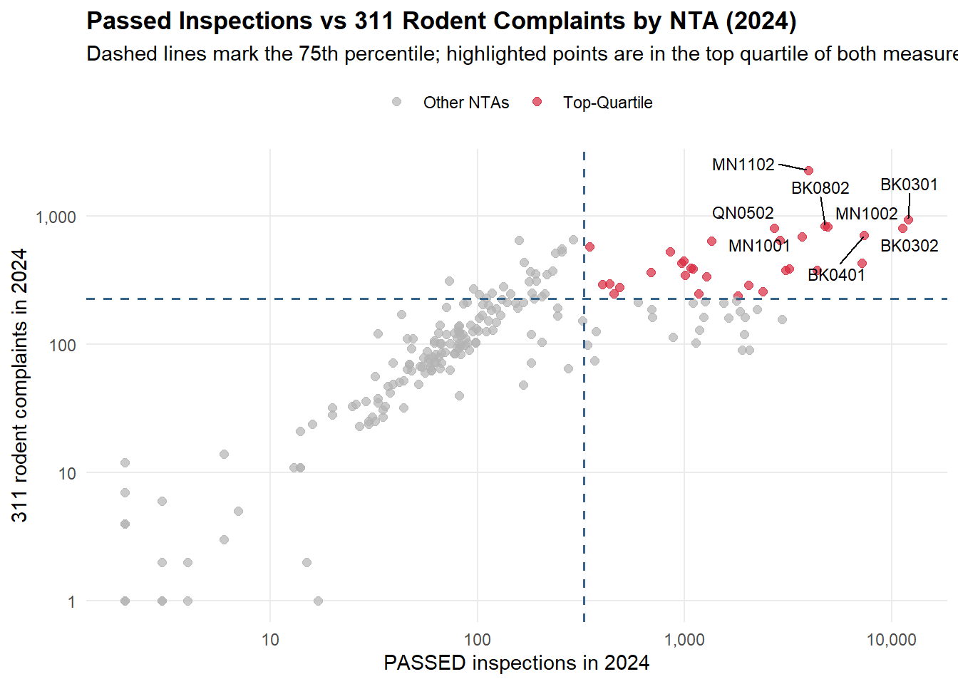
The table above presents NTAs that fall at or above the 75th percentile for both passed rodent inspections and 311 rodent-related complaint counts in 2024. By restricting to neighborhoods that rank high on both measures, the table highlights areas where frequent inspection activity co-occurs with high levels of resident reporting that year. The data indicates a presence of NTAs with elevated complaint volumes despite a large number of passed inspections in areas like Bedford-Stuyvesant.
Code
# Create flags (including mismatch) ONCEx_cut <-quantile(pass_call_2024$n_pass_2024, 0.75, na.rm =TRUE)y_cut <-quantile(pass_call_2024$calls_2024, 0.75, na.rm =TRUE)df <- pass_call_2024 %>%mutate(high_pass = n_pass_2024 >= x_cut,high_calls = calls_2024 >= y_cut,mismatch = high_pass & high_calls,x = n_pass_2024 +1, # +1 so log scale works with zerosy = calls_2024 +1 )# Label only the top 8 mismatch NTAs by complaintslabel_df <- df %>%filter(mismatch) %>%slice_max(calls_2024, n =8)# Plotggplot(df, aes(x = x, y = y)) +geom_point(aes(color = mismatch), size =2, alpha =0.7) +geom_vline(xintercept = x_cut +1, linetype ="dashed", linewidth =0.6, color ="steelblue4") +geom_hline(yintercept = y_cut +1, linetype ="dashed", linewidth =0.6, color ="steelblue4") +geom_text_repel(data = label_df,aes(label = area_id),size =3,max.overlaps =Inf,color ="black",box.padding =0.3 ) +scale_x_log10(labels = comma) +scale_y_log10(labels = comma) +scale_color_manual(values =c("FALSE"="grey70", "TRUE"="#D7263D"),labels =c("FALSE"="Other NTAs", "TRUE"="Top-Quartile") ) +labs(title ="Passed Inspections vs 311 Rodent Complaints by NTA (2024)",subtitle ="Dashed lines mark the 75th percentile; highlighted points are in the top quartile of both measures",x ="PASSED inspections in 2024",y ="311 rodent complaints in 2024",color =NULL ) +theme_minimal() +theme(legend.position ="top",panel.grid.minor =element_blank(),plot.title =element_text(face ="bold") )
This plot shows a positive association between passed inspections and complaint volume at the NTA level, with top-quartile NTAs highlighted. Even so, since inspections are triggered by complaints, this pattern likely reflects inspection targeting rather than changes in rat conditions, underscoring the need for an event-based analysis.
Top Community Districts by passed inspections and their 311 complaint volume (2024).
Community District
Passed Inspections
311 Complaints
BK03
23,660
1,708
BK04
14,257
1,133
MN10
8,516
1,514
MN03
8,459
583
MN11
5,846
2,494
BK08
5,794
1,025
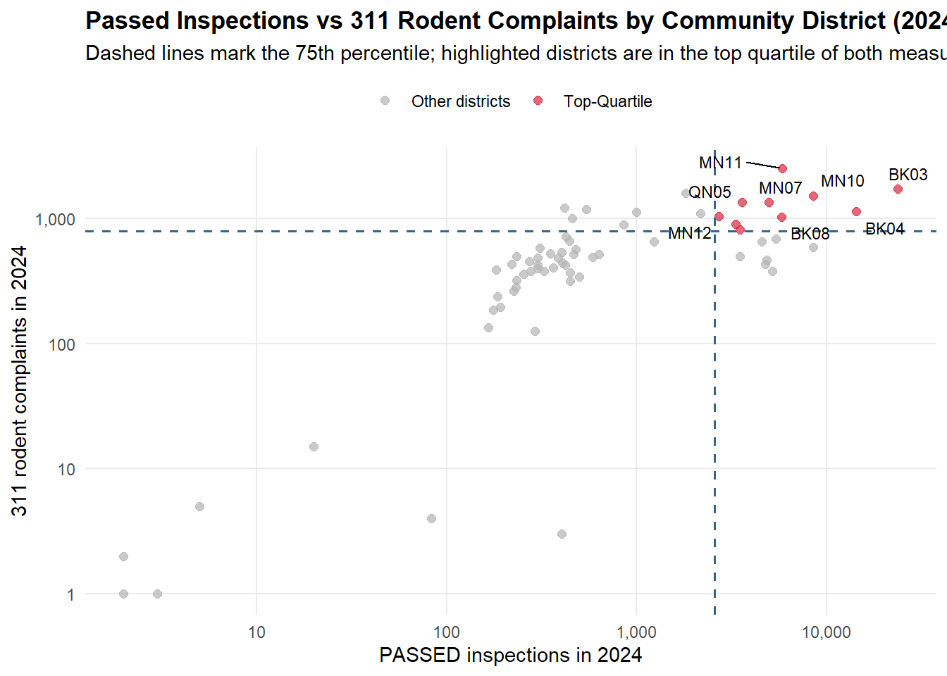
The same analysis was conducted at the Community District level. The table above presents Community Districts that fall at or above the 75th percentile for both passed rodent inspections and 311 rodent-related complaint counts in 2024. Brooklyn’s Community District 3 ranks at the top with 23,660 passed rodent inspections at 1,708 311 rodent complaints in 2024.
Code
# Flags + plotx_cut_cd <-quantile(pass_call_cd_2024$n_pass_2024, 0.75, na.rm =TRUE)y_cut_cd <-quantile(pass_call_cd_2024$calls_2024, 0.75, na.rm =TRUE)df_cd <- pass_call_cd_2024 %>%mutate(high_pass = n_pass_2024 >= x_cut_cd,high_calls = calls_2024 >= y_cut_cd,mismatch = high_pass & high_calls,x = n_pass_2024 +1,y = calls_2024 +1 )label_df_cd <- df_cd %>%filter(mismatch) %>%slice_max(calls_2024, n =8)# Plot itggplot(df_cd, aes(x = x, y = y)) +geom_point(aes(color = mismatch), size =2, alpha =0.7) +geom_vline(xintercept = x_cut_cd +1, linetype ="dashed",linewidth =0.6, color ="steelblue4") +geom_hline(yintercept = y_cut_cd +1, linetype ="dashed",linewidth =0.6, color ="steelblue4") +geom_text_repel(data = label_df_cd,aes(label = cd_id),size =3,max.overlaps =Inf,color ="black",box.padding =0.3 ) +scale_x_log10(labels = comma) +scale_y_log10(labels = comma) +scale_color_manual(values =c("FALSE"="grey70", "TRUE"="#D7263D"),labels =c("FALSE"="Other districts", "TRUE"="Top-Quartile") ) +labs(title ="Passed Inspections vs 311 Rodent Complaints by Community District (2024)",subtitle ="Dashed lines mark the 75th percentile; highlighted districts are in the top quartile of both measures",x ="PASSED inspections in 2024",y ="311 rodent complaints in 2024",color =NULL ) +theme_minimal() +theme(legend.position ="top",panel.grid.minor =element_blank(),plot.title =element_text(face ="bold") )
At the Community District level, complaint volume remains positively associated with inspection activity, reflecting inspection targeting. This descriptive pattern illustrates that aggregation preserves cross-sectional correlations but as said before, provides no insight into post-inspection dynamics, motivating the use of an event-based analysis.
Statistical Analysis Using Difference-in-Differences (DiD)
A weekly panel of rat-related 311 complaints by local area was constructed, and the week in which each neighborhood first received a passed inspection (referred to as PASS) was identified. An event-centered difference-in-differences design is adopted, in which time is indexed relative to the first passed inspection in each neighborhood. A Poisson regression with neighborhood fixed effects and an indicator for weeks following a passed inspection is estimated. The Poisson specification is appropriate given the count nature of the outcome and allows for a flexible mean–variance relationship while accommodating a large share of zero-valued observations. This specification compares changes in 311 complaint volume before and after a passed inspection within the same neighborhood, net of time-invariant neighborhood characteristics. Identification relies on the assumption that, absent a passed inspection, complaint trends within neighborhoods would have evolved similarly in the pre- and post-inspection periods.
DiD Model Estimates
All three specifications are estimated using the fixest package to maintain a consistent estimation framework across different spatial scales. In each case, the outcome is a count of rat-related 311 complaints aggregated to the relevant week. Models are estimated with fepois, which fits a fixed-effects Poisson regression via Poisson quasi–maximum likelihood while efficiently absorbing high-dimensional fixed effects. This approach is well suited to complaint counts that are nonnegative and often zero, and it allows unit fixed effects to be included without manually creating large sets of dummy variables. Across specifications, standard errors are clustered at the unit level to account for within-unit serial correlation in complaint activity over time.
150m Radius Model
First, the DiD model was run at the 150-meter spatial radius, and the results are shown below.
Code
# Fit Poisson DiD model using fixed-effects Poisson using fixest packagem150_w <-fepois( calls_w ~ post_pass_w | neigh_id_w,data = panel_neigh_w,vcov =~ neigh_id_w)tidy_m150 <-tidy(m150_w) |>filter(term =="post_pass_w") |>transmute(Estimate =round(estimate, 3),`Std. Error`=round(std.error, 3),`P-value`=ifelse(p.value <0.001, "< 0.001", round(p.value, 3)) )tidy_m150 |>kable(caption ="Effect of Passed Inspections on Weekly 311 Complaints (150-meter radius)",align ="c" ) |>kable_styling(full_width =FALSE)
Effect of Passed Inspections on Weekly 311 Complaints (150-meter radius)
Estimate
Std. Error
P-value
-1.135
0.017
< 0.001
The DiD estimate indicates a statistically significant decline in complaints following a passed inspection (β = −1.135, SE = 0.017, p < 0.001). This result suggests that, at a highly localized spatial scale, passed inspections are associated with a meaningful short-run reduction in resident-reported rodent activity.
NTA Model
Next, the DiD model was run at the NTA spatial scale, and the results are shown below.
Effect of Passed Inspections on 311 Complaints (NTA level)
Estimate
Std. Error
P-value
-0.369
0.419
0.378
In contrast to the highly localized 150-meter analysis, the estimated effect at the NTA scale is negative but not statistically significant (β = −0.369, SE = 0.419, p = 0.378). This result suggests that when inspection outcomes and complaints are aggregated to broader neighborhood boundaries, any localized reduction in complaint activity following a passed inspection is no longer detectable.
Community District Model
Lastly, the DiD model was ran at the Community District spatial scale and the results are below.
Effect of Passed Inspections on 311 Complaints (Community District Level)
Estimate
Std. Error
P-value
18.484
0
< 0.001
Unlike the NTA-level results, the estimated effect at this broader spatial scale is positive and statistically significant (β = 18.484, p < 0.001). However, this estimate should be interpreted with caution. The small number of observations (34 Community Districts) and the resulting zero reported standard error suggest that the model is operating at the limits of what can be reliably estimated at this level of aggregation.
Model Validation
Before presenting the main estimates, diagnostic checks were considered to assess the plausibility of the identifying assumptions.
Stable Unit Treatment Value Assumption (SUTVA)
Spillovers across neighborhoods are likely to be limited because rat inspections target specific properties and complaint reporting is highly localized. Residents typically report conditions in their immediate vicinity, making it unlikely that a passed inspection in one neighborhood directly affects complaint behavior in non-adjacent areas.
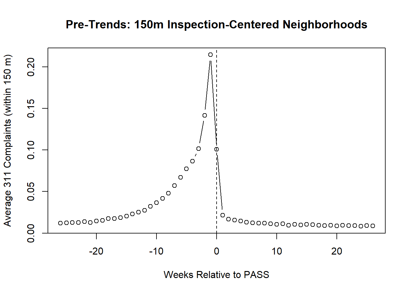
Event-time averages show a sharp increase in complaints immediately before a passed inspections, consistent with inspections being triggered by accumulated reports. Identification therefore relies on comparing post-inspection outcomes to the immediate pre-inspection period under a local parallel trends assumption. Following a passed inspection, complaint counts drop sharply and then stabilize, with no evidence of rebound. This concentration of effects in the immediate post-inspection period justifies the use of a short event window, as extending the window adds little information and primarily introduces noise.
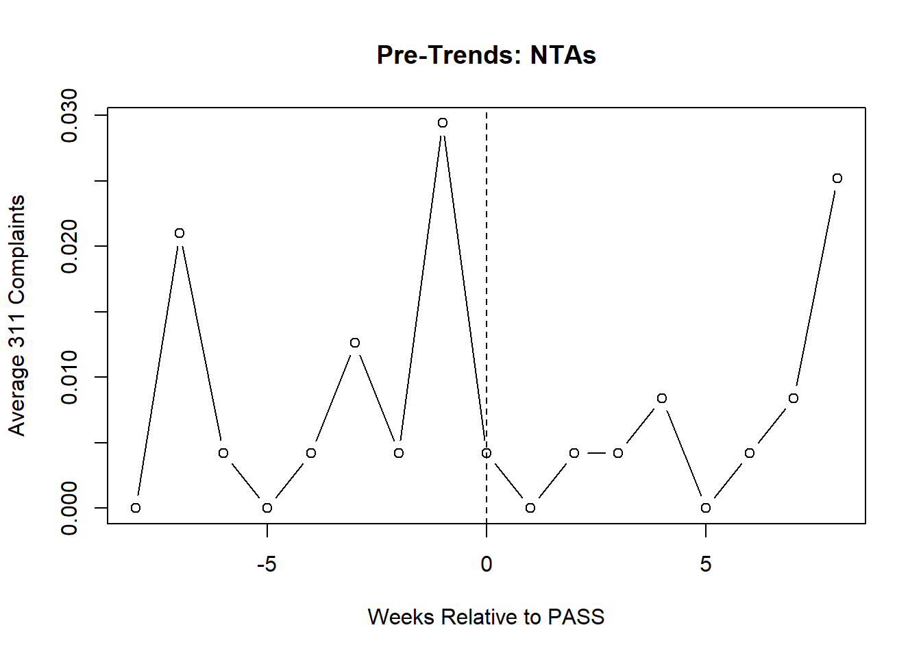
Event-time averages exhibit some week-to-week variability in the pre-inspection period, which is expected given low complaint counts and aggregation at the neighborhood level. However, there is no evidence of a systematic downward trend prior to PASS inspections. In addition, placebo timing tests yield null effects, providing no evidence of differential pre-trends.
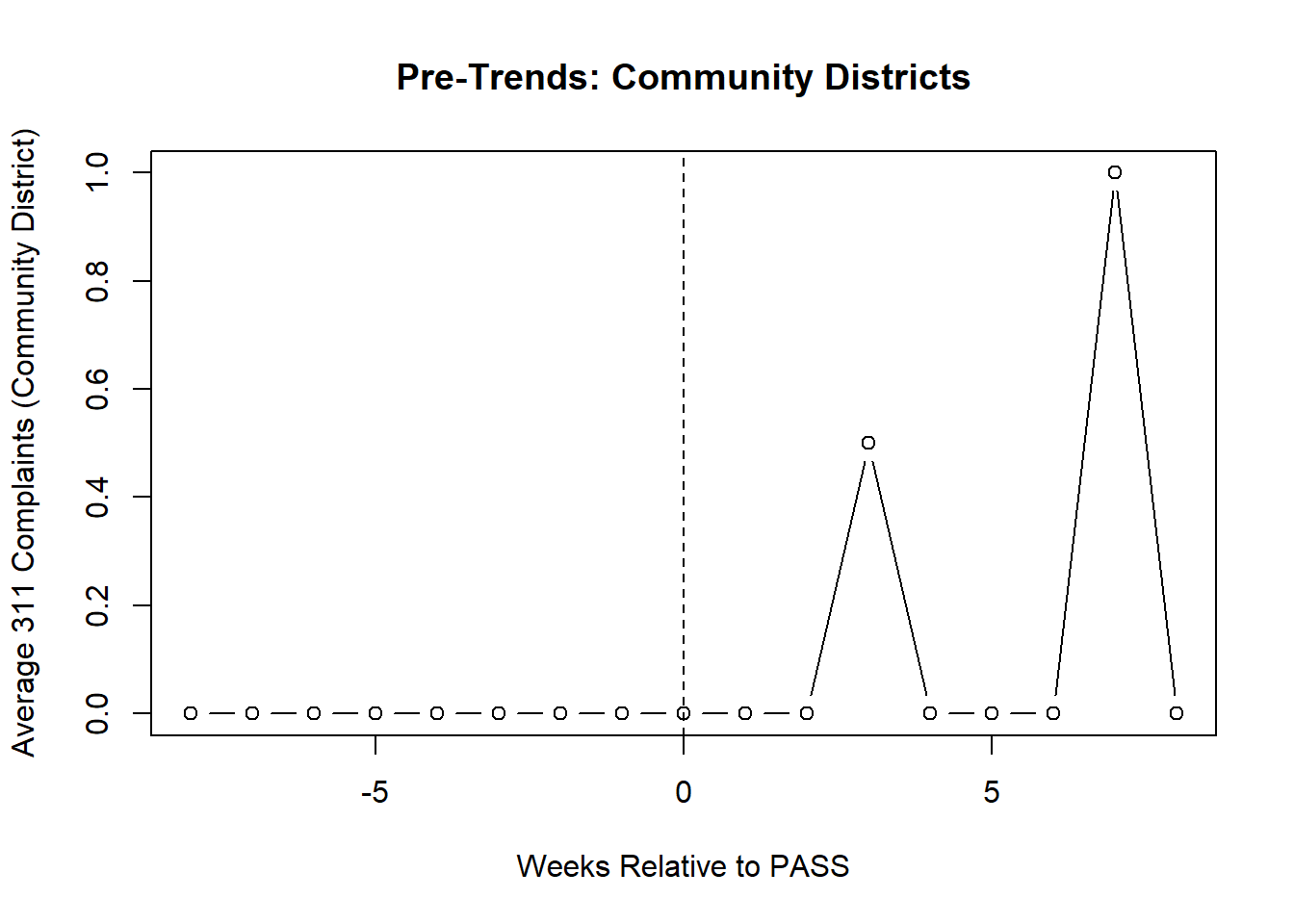
At the community district level, average complaint activity shows no pronounced pre-inspection pattern and remains close to zero prior to PASS inspections. This reflects the coarse spatial aggregation of community districts, within which localized inspection-related complaint dynamics are largely diluted.
Results
Raw coefficient results are not intuitive because Poisson was used in the model. Instead percentage changes can be reported using the following formula:
# helper to extract one coefficient row cleanlyone_term <-function(model, term) {tidy(model) |>filter(term ==!!term) |>transmute(beta = estimate,se = std.error,p = p.value )}# extract results from each modelcd <-one_term(m_cd, "post_pass_cd")nta <-one_term(m, "post_pass")r150 <-one_term(m150_w,"post_pass_w")# implied % change (Poisson): 100*(exp(beta)-1)pct_cd <-100* (exp(cd$beta) -1)pct_nta <-100* (exp(nta$beta) -1)pct_150 <-100* (exp(r150$beta)-1)# build a clean wide table with labeled rowstab <-tibble(Metric =c("Post-PASS (β)", "Std. Error", "P-value", "Implied % change (100×(exp(β)−1))"),`Community District`=c(sprintf("%.3f", cd$beta),sprintf("%.3f", cd$se),ifelse(cd$p <0.001, "< 0.001", sprintf("%.3f", cd$p)),"—"# CD implied % change is astronomically large / unstable; omit ),`NTA`=c(sprintf("%.3f", nta$beta),sprintf("%.3f", nta$se),ifelse(nta$p <0.001, "< 0.001", sprintf("%.3f", nta$p)),sprintf("%.1f%%", pct_nta) ),`150 m radius`=c(sprintf("%.3f", r150$beta),sprintf("%.3f", r150$se),ifelse(r150$p <0.001, "< 0.001", sprintf("%.3f", r150$p)),sprintf("%.1f%%", pct_150) ))tab |>kable(caption ="Effect of Passed Inspections on 311 Complaints Across Spatial Scales (2024)",align =c("l", "c", "c", "c") ) |>kable_styling(full_width =FALSE)
Effect of Passed Inspections on 311 Complaints Across Spatial Scales (2024)
Metric
Community District
NTA
150 m radius
Post-PASS (β)
18.484
-0.369
-1.135
Std. Error
0.000
0.419
0.017
P-value
< 0.001
0.378
< 0.001
Implied % change (100×(exp(β)−1))
—
-30.9%
-67.9%
This table reports the difference-in-differences estimates of the effect of PASS inspections on rat-related 311 complaints across all three spatial scales. At the community district level, the estimated effect is small and statistically indistinguishable from zero, reflecting substantial spatial dilution. Estimates at the NTA level are larger in magnitude but imprecise. In contrast, inspection-centered neighborhoods defined within a 150 m radius exhibit a large and statistically significant decline in complaints following a PASS inspection, consistent with highly localized treatment effects.
95% Confidence Intervals by Spatial Scale
Code
# Helper: convert log effect + SE into percent change + 95% intervalto_pct_ci <-function(beta, se, z =1.96) { lo <- beta - z * se hi <- beta + z * sec(estimate_pct = (exp(beta) -1) *100,lower_pct = (exp(lo) -1) *100,upper_pct = (exp(hi) -1) *100 )}# 1) Community Districts: fepoisb_cd <-coef(m_cd)[["post_pass_cd"]]se_cd <-se(m_cd)[["post_pass_cd"]]ci_cd <-to_pct_ci(b_cd, se_cd)# 2) 150m: fepoisb_150 <-coef(m150_w)[["post_pass_w"]]se_150 <-se(m150_w)[["post_pass_w"]]ci_150 <-to_pct_ci(b_150, se_150)# 3) NTA: fepois (your object m is also fepois)b_nta <-coef(m)[["post_pass"]]se_nta <-se(m)[["post_pass"]] # <-- FIX: use se(m), not coef(m)ci_nta <-to_pct_ci(b_nta, se_nta)# Combine + format nicelyresults_all <-tibble(Scale =c("150 m radius", "NTA", "Community District"),`Estimated % change`=c(ci_150["estimate_pct"], ci_nta["estimate_pct"], ci_cd["estimate_pct"]),`95% CI (lower)`=c(ci_150["lower_pct"], ci_nta["lower_pct"], ci_cd["lower_pct"]),`95% CI (upper)`=c(ci_150["upper_pct"], ci_nta["upper_pct"], ci_cd["upper_pct"])) |>mutate(across(-Scale, ~round(.x, 1))) |>mutate(`Estimated % change`=paste0(`Estimated % change`, "%"),`95% CI (lower)`=paste0(`95% CI (lower)`, "%"),`95% CI (upper)`=paste0(`95% CI (upper)`, "%") )results_all |>kable(caption ="Estimated percent change in 311 complaints after a passed inspection (with 95% confidence intervals)",align =c("l", "c", "c", "c") ) |>kable_styling(full_width =FALSE, bootstrap_options =c("striped", "hover"))
Estimated percent change in 311 complaints after a passed inspection (with 95% confidence intervals)
Scale
Estimated % change
95% CI (lower)
95% CI (upper)
150 m radius
-67.9%
-68.9%
-66.8%
NTA
-30.9%
-69.6%
57.1%
Community District
10652785848.9%
10652764969.5%
10652806728.4%
The estimated percent change in weekly 311 rodent complaint counts following a passed inspection are presented, along with 95% confidence intervals, across three spatial scales. At the most localized level, the estimated effect is a large and statistically significant reduction in complaints (−67.9%), with a narrow confidence interval that lies entirely below zero. This indicates a consistent short-run decline in complaint activity in the immediate vicinity of a passed inspection.
At the NTA level, the estimated effect remains negative (−30.9%) but is substantially less precise, as reflected in a wide confidence interval that spans both negative and positive values. This lack of precision suggests that any localized post-inspection decline in complaints is diluted when outcomes are aggregated to broader neighborhood boundaries.
In contrast, the Community District–level estimate implies an extremely large positive percent change, with a correspondingly narrow confidence interval. This result should be interpreted with caution, as it reflects aggregation effects and model instability at a coarse spatial scale rather than a plausible causal increase in rodent complaints following inspections. The results highlight strong scale dependence in estimated post-inspection effects and underscore the importance of spatial resolution when using 311 complaint data to assess changes in rodent activity.
Discussion
Key Findings: Connection to the Overarching Question
311 rodent complaints reflect rat activity only at highly localized spatial scales. Within 150 meters of a passed inspection, complaint volumes decline sharply and significantly, indicating that fine-scale 311 data capture real, localized changes in rat conditions.
Spatial aggregation weakens and distorts this relationship. At the NTA level, post-inspection effects become statistically insignificant, and at the Community District level estimates are unstable, reflecting spatial dilution rather than meaningful changes in rat activity.
Community District–level complaints primarily measure reporting behavior, not rat prevalence. When aggregated to administrative boundaries, 311 complaint counts blend heterogeneous neighborhoods and reporting tendencies, allowing high complaint volumes to persist despite frequent passed inspections and obscuring true ecological risk.
Recommendations for Research and Policy
Reconsider the use of Community District–level 311 complaints in Rat Mitigation Zones. Aggregating rodent complaints at the Community District level obscures localized rat activity and emphasizes reporting behavior. Using these counts to designate or evaluate Rat Mitigation Zones risks misidentifying high-reporting areas as high-risk areas.
Prioritize fine-scale complaint metrics for policy targeting. City agencies should rely on more localized measures—such as complaint density within small buffers around inspection sites or blocks—to better align data with how rat activity and inspections operate on the ground.
Treat spatial scale as a core design choice in future research. Researchers using 311 complaints should test sensitivity across multiple spatial resolutions and avoid causal claims based on highly aggregated data. Combining 311 complaints with inspection outcomes and environmental indicators can help separate true rat risk from reporting behavior.
Conclusion
In conclusion, this analysis demonstrates that the usefulness of 311 rodent complaints depends on spatial scale. At highly localized levels, complaints respond to passed inspections and reflect real changes in rat conditions. When aggregated to broader units such as Community Districts, complaint counts are dominated by reporting behavior rather than ecological risk. These findings caution against relying on aggregated 311 data for policy decisions like Rat Mitigation Zone designation and emphasize the need to align analytic scale with the localized nature of urban rat activity.
Source Code
---title: "When 311 Complaints Stop Measuring NYC Rats"subtitle: "Identifying Bias in Spatial Scales Using Statistical Analysis"author: "Sojung Chu"date: 2025-12-18date-format: "MMMM D, YYYY"format: html: code-tools: true code-fold: true toc: true toc-location: right number-sections: false toc-depth: 3 df-print: paged # runtime: shinyexecute: eval: true echo: true warning: false message: falsebibliography: individual_report.bibcsl: apa.csl---{width=25%}# IntroductionThis report is my individual component of a [group final course project](https://shreyakarki71.github.io/STA9750-2025-FALL/final_project.html) with [Shreya](https://shreyakarki71.github.io/STA9750-2025-FALL/individual_report.html), [Rachel](https://rcutsumpas-cloud.github.io/STA9750-2025-FALL/docs/rats_analysis_demo.html), [Geraldine](https://ghirschhorn.github.io/STA9750-2025-FALL/final.html), [David](https://samsmadge.github.io/STA9750-2025-FALL/individual_report.html), and [Wing](https://git4wing.github.io/STA9750-2025-FALL/Final_individual.html#introduction). Initially, we wanted to solve the case of the pesky rats that rule over New York City (NYC) by finding a correlation between the 311 rodent complaints, which are often used as markers for where the rats are located, and other factors. While much of the existing research focuses on identifying the factors that lead to rat infestations, our study instead examined whether 311 rodent complaints are an accurate proxy for rat prevalence. We investigated whether reliance on 311 data introduces bias.> **Specific Research Question: Does spatial aggregation cause 311 rodent calls to reflect reporting behavior rather than rat activity?**My analysis addresses whether spatial aggregation causes rodent complaints to reflect reporting behavior rather than rat activity. In 2017, NYC began designating [Rat Mitigation Zones](https://codelibrary.amlegal.com/codes/newyorkcity/latest/NYCrules/0-0-0-138869), with one criterion being the number of rat-related 311 complaints at the community district level. A difference-in-differences approach was used to compare 311 rodent complaints before and after a rodent inspection, with a passed inspection treated as the event at time zero. With inferring that a passed inspection signals acceptable rat conditions, we expect complaints to decline within the spatial unit after a passed inspection, provided the unit accurately captures rodent activity. This expectation was evaluated at three spatial scales: a local 150‑meter radius, Neighborhood Tabulation Areas (NTA) to maintain consistency with my groupmate’s analysis, and Community Districts to align with how NYC aggregates 311 rat complaints.The technical details of the analysis, including data acquisition, data cleaning, exploratory data analysis, and model estimation, are documented in this report. Reproducible code and detailed explanations illustrating how difference-in-differences models were developed and evaluated using NYC data are also included. All analyses were conducted in R through associated packages.# MethodologyThe following methods were used to obtain and reconstruction four datasets to prepare for analysis.## Data AcquisitionData was downloaded responsibly through functions that only download the required data if it does not already exist. Before this, the process starts by loading necessary packages through a helper function that installs and loads R packages used throughout this report. ```{r}#' Install and load an R package if it is not already available.#'#' @param pkg A character string specifying the name of the package to load.#' @return Invisibly returns TRUE if the package is successfully loaded.#' @examples#' load_package("tidyr")load_package <-function(pkg) {if (!requireNamespace(pkg, quietly =TRUE)) {install.packages(pkg) }suppressPackageStartupMessages(library(pkg, character.only =TRUE))}PACKAGES <-c("httr2", "jsonlite", "dplyr", "sf", "purrr", "tidyr", "broom","lubridate", "readr", "tidyverse", "nngeo", "ggplot2", "fixest", "nngeo", "scales","knitr", "ggrepel", "kableExtra", "shiny", "leaflet", "data.table", "modelsummary").loaded <-lapply(PACKAGES, load_package)```### Rodent InspectionsThe NYC Rat Inspection dataset contains records of rodent inspections conducted across the five boroughs in response to public complaints and routine monitoring. This dataset is compiled and published by the New York City Department of Health and Mental Hygiene (DOHMH) and is publicly available through [NYC Open Data](https://data.cityofnewyork.us/Health/Rodent-Inspection/p937-wjvj/about_data). The dataset contains approximately 2.9 million records, with a small number of inspections dated between 1918 and 1971 and two records from 2000, but these early outliers were removed. The majority of observations begin on January 1, 2001, and extend through December 8, 2025. Each record represents an individual inspection and includes information such as the inspection date, inspection outcome, and location details. Some records list inspection dates in 2045. These future-dated entries were identified as data errors and were removed. ```{r}#' Download and cache NYC rat inspection records from NYC Open Data.#'#' This chunk defines a helper function that retrieves rat inspection records from the#' NYC Open Data API and stores a local cached copy for reuse in future runs. Because#' the dataset can exceed single-request limits, the function downloads the data in#' paginated batches using `$limit` and `$offset`, combines the batches into a single#' table, and saves the result as a CSV in the project data directory. If a cached file#' already exists and `refresh = FALSE`, the function reads the local CSV instead of#' re-downloading the data.#'#' @return A tibble containing the full set of rat inspection records returned by the#' NYC Open Data endpoint.#' @examples#' rat_inspection <- load_rat_inspection()# Ensure a local directory exists for storing cached API downloads.# Caching downloaded files allows the analysis to be rerun without# repeatedly querying the NYC Open Data API.if (!dir.exists("data/final")) {dir.create("data/final", showWarnings =FALSE, recursive =TRUE)}load_rat_inspection <-function(refresh =FALSE) {# Define a local cache path so the dataset can be reused across runs.# Caching avoids repeated API calls and makes the workflow reproducible. target_dir <-"data/final" f_name <-"rat_inspection.csv" file_path <-file.path(target_dir, f_name)# Create the cache directory if it does not already exist.if (!dir.exists(target_dir)) {dir.create(target_dir, recursive =TRUE) }# If no cached file is available, or if a refresh is requested, download the data.# Otherwise, read the previously saved file from disk.if (!file.exists(file_path) || refresh) {message("Downloading full rat inspection dataset from NYC Open Data...")# Specify the NYC Open Data endpoint used to retrieve the inspection records. base_url <-"https://data.cityofnewyork.us/resource/p937-wjvj.json"# The Socrata API limits the number of rows returned per request, so the full# dataset is retrieved in repeated chunks using limit and offset parameters. chunk_limit <-50000L all_chunks <-list() offset <-0L chunk_id <-1Lrepeat {message("Requesting rows with offset = ", offset, " ...") resp <-request(base_url) |>req_url_query("$limit"= chunk_limit,"$offset"= offset ) |>req_perform()# Stop execution if the API request fails.resp_check_status(resp)# Parse the response into a tabular object that can be combined across chunks.# Flattening is used to bring nested fields into regular columns when present. raw_json <-resp_body_string(resp) dat_list <-fromJSON(raw_json, flatten =TRUE) chunk_tbl <- dat_list |>as_tibble() n_chunk <-nrow(chunk_tbl)message("Retrieved ", n_chunk, " rows in chunk ", chunk_id, ".")# A zero-row response indicates the end of the export.if (n_chunk ==0) {message("No more rows returned. Reached end of dataset.")break } all_chunks[[chunk_id]] <- chunk_tbl# If the chunk is smaller than the request limit, assume this is the final page.if (n_chunk < chunk_limit) {message("Final chunk returned fewer than ", chunk_limit, " rows.")break }# Otherwise, advance the offset and request the next batch. offset <- offset + n_chunk chunk_id <- chunk_id +1L }# Combine all retrieved chunks into a single table. rat_inspection <-bind_rows(all_chunks)message("Total rows downloaded: ", nrow(rat_inspection))# Save the assembled dataset so it can load it from disk.write_csv(rat_inspection, file_path) } else {message("Reading existing rat inspection data from CSV...") rat_inspection <-read_csv(file_path, show_col_types =FALSE) } rat_inspection}rat_inspection <-load_rat_inspection()# Filter out inspection records with implausible dates that likely reflect data issues.# This removes a small number of records dated 1918–1971, the two records from 2000,# and outliers dated in 2045.rat_inspection <- rat_inspection |>mutate(inspection_date =as_date(inspection_date)) |>filter(!is.na(inspection_date)) |>filter(year(inspection_date) >=1972,year(inspection_date) <=2024) |>filter(year(inspection_date) !=2000)```### 311 Rodent ComplaintsThe New York City 311 Rodent Complaints data set contains records of service requests submitted by residents reporting rodent sightings. This dataset is compiled and made publicly available through the NYC Open Data portal and from the [NYC 311 service system](https://data.cityofnewyork.us/Social-Services/311-Rodent-Complaints/cvf2-zn8s/about_data). It contains approximately 492,000 records and spans from January 2010 through December 2025. Each record includes information such as the date the complaint was submitted, complaint type, and location details.```{r}#' Download and assemble NYC 311 rodent complaint records from NYC Open Data.#'#' This chunk prepares a local data directory and defines a helper function that#' retrieves NYC 311 rodent complaint data from the NYC Open Data API. Because the#' dataset can exceed single-request limits, the function downloads the data in#' paginated batches using `$limit` and `$offset`. Each batch is cached locally as#' a GeoJSON file to avoid repeated downloads and to make the workflow reproducible.#' The cached batches are then read with `st_read()` and combined into a single dataset.#'#' @return An `sf` object containing the full set of rodent complaint records returned#' by the NYC Open Data endpoint.#' @examples#' rodent_complaints <- get_rodent_complaints()# Define a helper function to download and assemble NYC 311 rodent complaint data.# The function retrieves the data in batches to accommodate API request limits,# caches each batch locally as a GeoJSON file, and combines all batches into# a single sf object for downstream analysis.get_rodent_complaints <-function() {# Define the NYC Open Data API endpoint for 311 rodent complaints.# The data are served as GeoJSON and must be retrieved in multiple requests. ENDPOINT <-"https://data.cityofnewyork.us/resource/cvf2-zn8s.geojson" BATCH_SIZE <-50000 OFFSET <-0 END_OF_EXPORT <-FALSE FILE_INDEX <-1 ALL_DATA <-list()# Continue requesting data until the API returns fewer rows than the batch size,# which signals that the end of the dataset has been reached.while (!END_OF_EXPORT) {# Construct a stable filename for the current batch so that it can be reused# across multiple runs of the analysis. file_name <-sprintf("rodent_311_%04d.geojson", FILE_INDEX) file_path <-file.path("data/final", file_name)# Download the current batch only if it has not already been saved locally.# This avoids unnecessary API calls and improves reproducibility.if (!file.exists(file_path)) { req <-request(ENDPOINT) |>req_url_query(`$limit`= BATCH_SIZE,`$offset`= OFFSET ) resp <-req_perform(req)resp_check_status(resp)resp_body_raw(resp) |>writeBin(con = file_path) }# Read the cached GeoJSON batch into an sf object. batch_data <-st_read(file_path, quiet =TRUE)# Append the current batch to the list of all downloaded data. ALL_DATA <-c(ALL_DATA, list(batch_data))# If the number of returned rows is smaller than the requested batch size,# the final page has been reached and the loop can terminate.if (NROW(batch_data) != BATCH_SIZE) { END_OF_EXPORT <-TRUE } else { OFFSET <- OFFSET + BATCH_SIZE FILE_INDEX <- FILE_INDEX +1 } }# Combine all downloaded batches into a single sf object. ALL_DATA <-bind_rows(ALL_DATA)return(ALL_DATA)}# Execute the data download and combination step and store the result.rodent_complaints <-get_rodent_complaints()```### Neighborhood Tabulation Areas (NTA)The 2020 [New York City Neighborhood Tabulation Area](https://www.nyc.gov/content/planning/pages/resources/datasets/neighborhood-tabulation) (NTA) boundary polygons were downloaded from an ArcGIS REST service provided by the City of New York. These polygons define standardized neighborhood units commonly used for demographic and public health analyses. The boundary file was cached locally to ensure reproducibility and loaded as a spatial object, then transformed to align with the rodent inspection and 311 complaint data.```{r}#' Download and load NYC Neighborhood Tabulation Area (NTA) boundary polygons.#'#' This function downloads the 2020 Neighborhood Tabulation Area boundary polygons from an#' ArcGIS REST endpoint and caches the GeoJSON locally for reuse. If the file already exists#' locally, it is read from disk instead of being downloaded again.#' The boundaries are loaded as an `sf` object and transformed to EPSG:4326 to align with#' the coordinate reference system used by the rodent datasets.#'#' @param nta_url URL of the ArcGIS GeoJSON endpoint (default provided).#' @param nta_path Local filepath used to cache the downloaded GeoJSON.#' @return An `sf` object containing NYC Neighborhood Tabulation Area polygon geometries#' and associated attributes.#' @importFrom httr2 request req_perform resp_check_status resp_body_raw#' @importFrom sf st_read st_transform#' @exportload_nta_boundaries <-function(nta_url ="https://services5.arcgis.com/GfwWNkhOj9bNBqoJ/arcgis/rest/services/NYC_Neighborhood_Tabulation_Areas_2020/FeatureServer/0/query?where=1=1&outFields=*&outSR=4326&f=pgeojson",nta_path ="data/final/nta_2020.geojson",refresh =FALSE) {# Ensure the output directory exists before attempting to write cached files. out_dir <-dirname(nta_path)if (!dir.exists(out_dir)) {dir.create(out_dir, recursive =TRUE) }# Download the file only if it is not already cached locally.# This keeps the workflow reproducible and avoids repeated requests to the server.if (!file.exists(nta_path)) { resp <-request(nta_url) |>req_perform()resp_check_status(resp)resp_body_raw(resp) |>writeBin(con = nta_path) }# Read the cached NTA boundaries as an sf object and standardize the CRS.# Using a consistent CRS ensures spatial joins and distance calculations work as expected. nta <-st_read(nta_path, quiet =TRUE) |>st_transform(4326)return(nta)}nta <-load_nta_boundaries()```### Community DistrictsThe New York City [Community District](https://www.nyc.gov/content/planning/pages/resources/datasets/community-districts) boundary polygons were downloaded from the NYC Department of City Planning’s dataset, using an ArcGIS REST endpoint that provides the boundaries in GeoJSON format. The boundary file was also cached locally.```{r}#' Download and load NYC Community District boundary polygons.#'#' This function downloads NYC Department of City Planning Community District boundaries#' from an ArcGIS REST endpoint and caches the GeoJSON locally for reuse. If the file#' already exists locally, it is read from disk instead of being downloaded again. #' The boundaries are loaded as an `sf` object and transformed to to ensure compatibility#' with other datasets used in the analysis.#'#' @param cd_url URL of the ArcGIS GeoJSON endpoint (default provided).#' @param cd_path Local filepath used to cache the downloaded GeoJSON#' (default "data/final/community_districts.geojson").#' @return An `sf` object containing Community District polygons. The returned object#' includes the Community District identifier (`BoroCD`) and geometry.#' @importFrom httr2 request req_perform resp_check_status resp_body_raw#' @importFrom sf st_read st_transform#' @importFrom dplyr select#' @exportload_cd_shapefiles <-function(cd_url ="https://services5.arcgis.com/GfwWNkhOj9bNBqoJ/arcgis/rest/services/NYC_Community_Districts/FeatureServer/0/query?where=1=1&outFields=*&outSR=4326&f=pgeojson",cd_path ="data/final/community_districts.geojson",refresh =FALSE) {# Ensure the output directory exists before attempting to write cached files. out_dir <-dirname(cd_path)if (!dir.exists(out_dir)) {dir.create(out_dir, recursive =TRUE) }# Download the GeoJSON only when needed to minimize repeated server requests.if (refresh ||!file.exists(cd_path)) { resp <-request(cd_url) |>req_perform()resp_check_status(resp)resp_body_raw(resp) |>writeBin(con = cd_path) }# Read the cached GeoJSON and standardize to EPSG:4326 for spatial compatibility. cd <-st_read(cd_path, quiet =TRUE) |>st_transform(4326)# Keep only the Community District identifier and geometry used for joins. cd <- cd |>select(BoroCD, geometry)return(cd)}cd_keep <-load_cd_shapefiles()```## Data IntegrationSince the rodent inspection and 311 complaint data are recorded at the point level using latitude and longitude coordinates, I standardized the geographic unit of analysis across the 311 rodent complaint and rodent inspection datasets. Point locations were converted to spatial features and spatially joined to 2020 NTA boundary polygons using a point-in-polygon approach, assigning each record to an NTA. ```{r}# Convert rodent complaint coordinates into sf point features.# Extract longitude and latitude as numeric values and remove records without valid coordinates.rat_coords <- rodent_complaints |>mutate(lon =as.numeric(longitude),lat =as.numeric(latitude) ) |>drop_na(lon, lat)# Convert the complaint records into an sf object so spatial operations can be applied.rats_sf <-st_as_sf( rat_coords,coords =c("lon", "lat"),crs =4326)# Load the NTA polygon boundaries and make sure they are in the same CRS as the complaint points.nta <-st_read("data/final/nta_2020.geojson", quiet =TRUE) |>st_transform(4326)# Create a lookup table mapping NTA names to official NTA codes for later joins.nta_lookup <- nta |>st_drop_geometry() |>select(nta = NTAName, nta_code = NTA2020 ) |>distinct()# Spatial join NTA attributes onto each complaint point.rat311_with_nta <-st_join( rats_sf, nta[, c("NTA2020", "NTAName", "BoroName")])# Drop geometry to work with a regular tabular data frame while keeping the NTA attributes.rat311_with_nta_df <- rat311_with_nta |>st_drop_geometry()```Community district polygons were then joined in a similar way.```{r}# Spatial join: assign each 311 rat point to a Community District (BoroCD)rat311_with_cd <-st_join(rats_sf, cd_keep)# Drop geometry for a regular tibblerat311_with_cd_df <- rat311_with_cd |>st_drop_geometry()# Drop geometry for a regular tabular data framerat311_with_cd_df <- rat311_with_cd |>st_drop_geometry()# Add Community District (BoroCD) to any NYC dataset with lon/lat columns# Keeps pipeline modular: load raw data first, enrich later, without modifying originals.add_cd_to_points <-function(df,lon_col ="longitude",lat_col ="latitude",cd_path ="data/final/community_districts.geojson") {# Read/prepare Community District polygons (lightweight) cd_keep <-st_read(cd_path, quiet =TRUE) |>st_transform(4326) |>select(BoroCD, geometry)# Extract coords + drop missing df_coords <- df |>mutate(lon =as.numeric(.data[[lon_col]]),lat =as.numeric(.data[[lat_col]]) ) |>drop_na(lon, lat)# Convert to sf points df_sf <-st_as_sf(df_coords, coords =c("lon", "lat"), crs =4326)# Spatial join + return as regular tibble (no geometry column)st_join(df_sf, cd_keep, left =TRUE) |>st_drop_geometry()}rat_inspection_with_cd_df <-add_cd_to_points(rat_inspection)rat311_with_cd_df <-add_cd_to_points(rodent_complaints)```## Data ConstructionIn order to implement a event-centered difference-in-differences design, balanced panels were constructed around the timing of passed rodent inspections. For each spatial scale, inspection events were treated as the focal intervention, and 311 rodent complaints were organized relative to the first passed inspection within a given geographic unit. All panels were constructed at the weekly level and retain weeks with zero complaints.### 150 Meter Radius```{r}#' Construct distance-based difference-in-differences panels around PASS inspections.#'#' To support the distance-based difference-in-differences analysis, this chunk integrates#' 311 rodent complaint records with PASS inspection locations using a spatial proximity#' approach. Both datasets are converted to spatial point features and projected to a#' coordinate reference system that preserves distances in meters. This allows complaint#' activity to be measured within a fixed radius of each inspection site and enables#' spatial proximity to be incorporated directly into the DiD design.#'#' The resulting data structure supports neighborhood-by-month panels with zero-call#' months included and is used to estimate Poisson DiD models with neighborhood and#' month fixed effects.# Specify the radius, in meters, used to define complaints occurring near a PASS inspection.# This value determines the spatial scale at which inspection effects are evaluated.# -----------------------------# WEEK VERSION (separate names) + recommended filters# -----------------------------radius_m_w <-150window_w_w <-26week_start_w <-1# 1 = Monday, 7 = Sunday# 1) 311 calls -> sf points with weekcalls_sf_w <- rat311_with_nta_df %>%filter(!is.na(longitude), !is.na(latitude)) %>%mutate(created_date_w =as.Date(created_date),call_week_w =floor_date(created_date_w, "week", week_start = week_start_w) ) %>%st_as_sf(coords =c("longitude", "latitude"), crs =4326) %>%st_transform(3857)# 2) Inspections -> sf points with week (PASS centers)insp_sf_w <- rat_inspection %>%filter(!is.na(longitude), !is.na(latitude)) %>%mutate(inspection_date_w =ymd(inspection_date),inspection_week_w =floor_date(inspection_date_w, "week", week_start = week_start_w) ) %>%st_as_sf(coords =c("longitude", "latitude"), crs =4326) %>%st_transform(3857)pass_sf_w <- insp_sf_w %>%filter(result =="Passed") %>%arrange(inspection_week_w) %>%mutate(neigh_id_w =row_number(),first_pass_week_w = inspection_week_w )# 3) Nearest PASS for each call within radiusnn_out_w <-st_nn( calls_sf_w, pass_sf_w,k =1, maxdist = radius_m_w,returnDist =TRUE,progress =FALSE)calls_sf_w <- calls_sf_w %>%mutate(pass_row_w =map_int(nn_out_w$nn, ~if (length(.x) ==0) NA_integer_else .x[1]),dist_to_pass_m_w =map_dbl(nn_out_w$dist, ~if (length(.x) ==0) NA_real_else .x[1]),neigh_id_w =if_else(is.na(pass_row_w), NA_integer_, pass_sf_w$neigh_id_w[pass_row_w]) ) %>%select(-pass_row_w)# 4) Keep only calls within chosen radius of a PASScalls_near_w <- calls_sf_w %>%filter(!is.na(dist_to_pass_m_w) & dist_to_pass_m_w <= radius_m_w)# 5) Aggregate to neighborhood × week: count callscalls_neigh_week_w <- calls_near_w %>%st_drop_geometry() %>%group_by(neigh_id_w, call_week_w) %>%summarise(calls_w =n(), .groups ="drop")# PASS event info per neigh_id_wpass_info_w <- pass_sf_w %>%st_drop_geometry() %>%select(neigh_id_w, first_pass_week_w)# 6) FULL PANEL: all neighborhoods × all weeks (fill zeros) + event-time varsall_weeks_w <-seq(from =min(calls_neigh_week_w$call_week_w, na.rm =TRUE),to =max(calls_neigh_week_w$call_week_w, na.rm =TRUE),by ="week")# Only neighborhoods that actually get used (nearest for >=1 call within radius)all_neigh_w <-sort(unique(calls_near_w$neigh_id_w))full_neigh_panel_w <-expand.grid(neigh_id_w = all_neigh_w,call_week_w = all_weeks_w)panel_neigh_w <- full_neigh_panel_w %>%left_join(calls_neigh_week_w, by =c("neigh_id_w", "call_week_w")) %>%mutate(calls_w =replace_na(calls_w, 0L)) %>%left_join(pass_info_w, by ="neigh_id_w") %>%mutate(rel_week_w =as.integer((call_week_w - first_pass_week_w) /7),post_pass_w =as.integer(rel_week_w >=0) ) %>%filter(rel_week_w >=-window_w_w, rel_week_w <= window_w_w)# 7) Recommended filters (balanced window + drop all-zero centers)panel_neigh_w <- panel_neigh_w %>%group_by(neigh_id_w) %>%mutate(n_pre_w =sum(rel_week_w <0),n_post_w =sum(rel_week_w >=0),total_calls_w =sum(calls_w, na.rm =TRUE) ) %>%ungroup() %>%filter( n_pre_w >=1, n_post_w >=1, total_calls_w >0 ) %>%select(-total_calls_w)```A distance-based neighborhood radius was constructed around each passed inspection to capture localized responses in 311 complaints. A 150-meter radius was selected to reflect the spatial range over which an inspection could influence nearby complaint behavior while minimizing spillovers from unrelated areas. Each complaint was linked to its nearest passed inspection within this radius, creating inspection-centered neighborhoods that remain fixed over time. Complaint counts were aggregated weekly, and a balanced panel was constructed around the inspection event.### NTA Level```{r}# Aggregate 311 calls weekly so each NTA has number of calls per week# 1) Weekly calls by NTA x calendar week (same as you have)calls_weekly <- rat311_with_nta_df %>%mutate(week =floor_date(created_date, "week", week_start =1),area_id = NTA2020 ) %>%filter(!is.na(area_id)) %>%group_by(area_id, week) %>%summarise(calls =n(), .groups ="drop")# 2) First PASS week per NTA (same logic, but keep pass_week + treat_start_week)pass_times <- rat_inspection %>%mutate(area_id = nta_code, pass_date = inspection_date) %>%filter(!is.na(area_id), result =="Passed", !is.na(pass_date)) %>%group_by(area_id) %>%summarise(first_pass_date =min(pass_date),pass_week =floor_date(first_pass_date, "week", week_start =1),treat_start_week = pass_week +weeks(1),.groups ="drop" )# 3) Build event-centered grid: NTA x rel_weekevent_grid <-expand.grid(area_id =unique(pass_times$area_id),rel_week =-8:8)# 4) Map each rel_week to the corresponding calendar week for that NTApanel_event <- event_grid %>%left_join(pass_times, by ="area_id") %>%mutate(week = treat_start_week +weeks(rel_week),post_pass =ifelse(rel_week >=0, 1L, 0L) ) %>%left_join(calls_weekly, by =c("area_id", "week")) %>%mutate(calls =replace_na(calls, 0L))# Optional Sanity checks# nrow(panel)# nlevels(panel$area_factor); nlevels(panel$month_factor)# table(panel$post_pass)```311 rodent complaints and inspection data were aggregated to weekly counts within each Neighborhood Tabulation Area (NTA), and inspection records were used to identify the first passed rodent inspection in each NTA with a 8-week window before and after. The first treatment period is defined to begin in the week following the inspection to avoid conflicting inspection-day reporting with post-inspection behavioral or environmental changes. An event-centered panel was constructed by expanding each NTA across a fixed window of relative weeks around the inspection event and merging in weekly complaint counts. ### Community District Level```{r}window_w <-8# 1) Weekly calls by CD x calendar weekcalls_weekly_cd <- rat311_with_cd_df %>%mutate(week_cd =floor_date(created_date, "week", week_start =1),cd_id =as.character(BoroCD) ) %>%filter(!is.na(cd_id), !is.na(week_cd)) %>%group_by(cd_id, week_cd) %>%summarise(calls_cd =n(), .groups ="drop")# 2) First PASS week by CD + treat_start_weekpass_times_cd <- rat_inspection_with_cd_df %>%mutate(cd_id =as.character(BoroCD),pass_date = inspection_date ) %>%filter(!is.na(cd_id), result =="Passed", !is.na(pass_date)) %>%group_by(cd_id) %>%summarise(first_pass_date_cd =min(pass_date),pass_week_cd =floor_date(first_pass_date_cd, "week", week_start =1),treat_start_week_cd = pass_week_cd +weeks(1),.groups ="drop" )# 3) Event-centered grid: CD x rel_weekevent_grid_cd <-expand.grid(cd_id =unique(pass_times_cd$cd_id),rel_week_cd =-window_w:window_w)# 4) Map rel_week -> calendar week, join calls, fill zerospanel_event_cd <- event_grid_cd %>%left_join(pass_times_cd, by ="cd_id") %>%mutate(week_cd = treat_start_week_cd +weeks(rel_week_cd),post_pass_cd =ifelse(rel_week_cd >=0, 1L, 0L) ) %>%left_join(calls_weekly_cd, by =c("cd_id", "week_cd")) %>%mutate(calls_cd =replace_na(calls_cd, 0L))# Drop CDs with all-zero calls in the windowpanel_event_cd <- panel_event_cd %>%group_by(cd_id) %>%filter(sum(calls_cd, na.rm =TRUE) >0) %>%ungroup()```As with the NTA analysis, a symmetric window was used and were aligned to event time, to enable direct comparison across spatial scales.# Exploratory Data Analysis## NTAs with Concurrent High Rodent Complaints and Passed Inspections (2024)```{r}passes_2024 <- rat_inspection %>%mutate(area_id = nta_code,inspection_date =ymd(inspection_date),year =year(inspection_date) ) %>%filter( year ==2024, result =="Passed",!is.na(area_id) ) %>%group_by(area_id) %>%summarise(n_pass_2024 =n(),.groups ="drop" ) %>%arrange(desc(n_pass_2024))calls_2024 <- rat311_with_nta_df %>%mutate(area_id = NTA2020,year =year(created_date) ) %>%filter( year ==2024,!is.na(area_id) ) %>%group_by(area_id) %>%summarise(calls_2024 =n(),.groups ="drop" ) %>%arrange(desc(calls_2024))pass_call_2024 <- passes_2024 %>%left_join(calls_2024, by ="area_id") %>%mutate(calls_2024 =replace_na(calls_2024, 0) ) %>%arrange(desc(n_pass_2024), desc(calls_2024))high_pass_threshold <-quantile(pass_call_2024$n_pass_2024, 0.75, na.rm =TRUE)high_call_threshold <-quantile(pass_call_2024$calls_2024, 0.75, na.rm =TRUE)suspicious_areas_2024 <- pass_call_2024 %>%mutate(high_pass = n_pass_2024 >= high_pass_threshold,high_calls = calls_2024 >= high_call_threshold,mismatch = high_pass & high_calls ) %>%filter(mismatch) %>%arrange(desc(n_pass_2024), desc(calls_2024))# Create table output using kableExtranta_lookup <- nta %>%st_drop_geometry() %>%transmute(area_id = NTA2020,nta_name = NTAName ) %>%distinct()pass_call_2024 %>%left_join(nta_lookup, by ="area_id") %>%slice_max(n_pass_2024, n =6, with_ties =FALSE) %>%transmute(`NTA Code`= area_id,`NTA Name`= nta_name,`Passed Rodent Inspections`=comma(n_pass_2024),`311 Rodent Complaints`=comma(calls_2024) ) %>%kable(align =c("l", "l", "r", "r"),caption ="High Number of Rodent Complaints and Passed Rodent Inspections (2024)" ) %>%kable_styling(full_width =FALSE, bootstrap_options =c("striped", "hover"))```The table above presents NTAs that fall at or above the 75th percentile for both passed rodent inspections and 311 rodent-related complaint counts in 2024. By restricting to neighborhoods that rank high on both measures, the table highlights areas where frequent inspection activity co-occurs with high levels of resident reporting that year. The data indicates a presence of NTAs with elevated complaint volumes despite a large number of passed inspections in areas like Bedford-Stuyvesant.```{r}# Create flags (including mismatch) ONCEx_cut <-quantile(pass_call_2024$n_pass_2024, 0.75, na.rm =TRUE)y_cut <-quantile(pass_call_2024$calls_2024, 0.75, na.rm =TRUE)df <- pass_call_2024 %>%mutate(high_pass = n_pass_2024 >= x_cut,high_calls = calls_2024 >= y_cut,mismatch = high_pass & high_calls,x = n_pass_2024 +1, # +1 so log scale works with zerosy = calls_2024 +1 )# Label only the top 8 mismatch NTAs by complaintslabel_df <- df %>%filter(mismatch) %>%slice_max(calls_2024, n =8)# Plotggplot(df, aes(x = x, y = y)) +geom_point(aes(color = mismatch), size =2, alpha =0.7) +geom_vline(xintercept = x_cut +1, linetype ="dashed", linewidth =0.6, color ="steelblue4") +geom_hline(yintercept = y_cut +1, linetype ="dashed", linewidth =0.6, color ="steelblue4") +geom_text_repel(data = label_df,aes(label = area_id),size =3,max.overlaps =Inf,color ="black",box.padding =0.3 ) +scale_x_log10(labels = comma) +scale_y_log10(labels = comma) +scale_color_manual(values =c("FALSE"="grey70", "TRUE"="#D7263D"),labels =c("FALSE"="Other NTAs", "TRUE"="Top-Quartile") ) +labs(title ="Passed Inspections vs 311 Rodent Complaints by NTA (2024)",subtitle ="Dashed lines mark the 75th percentile; highlighted points are in the top quartile of both measures",x ="PASSED inspections in 2024",y ="311 rodent complaints in 2024",color =NULL ) +theme_minimal() +theme(legend.position ="top",panel.grid.minor =element_blank(),plot.title =element_text(face ="bold") )```This plot shows a positive association between passed inspections and complaint volume at the NTA level, with top-quartile NTAs highlighted. Even so, since inspections are triggered by complaints, this pattern likely reflects inspection targeting rather than changes in rat conditions, underscoring the need for an event-based analysis.```{r}# Convert numeric BoroCD (e.g., 303) -> "BK03"to_cd_code <-function(borocd) { borocd <-as.integer(borocd) borough_num <- borocd %/%100 dist_num <- borocd %%100 borough_code <-case_when( borough_num ==1~"MN", borough_num ==2~"BX", borough_num ==3~"BK", borough_num ==4~"QN", borough_num ==5~"SI",TRUE~NA_character_ )paste0(borough_code, sprintf("%02d", dist_num))}# 2024 PASSED inspections by Community Districtpasses_cd_2024 <- rat_inspection_with_cd_df %>%mutate(cd_id =to_cd_code(BoroCD),year =year(inspection_date) ) %>%filter(year ==2024, result =="Passed", !is.na(cd_id)) %>%group_by(cd_id) %>%summarise(n_pass_2024 =n(), .groups ="drop")# 2024 311 rodent complaints by Community Districtcalls_cd_2024 <- rat311_with_cd_df %>%mutate(cd_id =to_cd_code(BoroCD),year =year(created_date) ) %>%filter(year ==2024, !is.na(cd_id)) %>%group_by(cd_id) %>%summarise(calls_2024 =n(), .groups ="drop")pass_call_cd_2024 <- passes_cd_2024 %>%left_join(calls_cd_2024, by ="cd_id") %>%mutate(calls_2024 =replace_na(calls_2024, 0L))pass_call_cd_2024 |>slice_max(n_pass_2024, n =6, with_ties =FALSE) |>mutate(n_pass_2024 =comma(n_pass_2024),calls_2024 =comma(calls_2024) ) |>kable(col.names =c("Community District", "Passed Inspections", "311 Complaints"),align =c("l", "r", "r"),caption ="Top Community Districts by passed inspections and their 311 complaint volume (2024)." ) |>kable_styling(full_width =FALSE, bootstrap_options =c("striped", "hover"))```The same analysis was conducted at the Community District level. The table above presents Community Districts that fall at or above the 75th percentile for both passed rodent inspections and 311 rodent-related complaint counts in 2024. Brooklyn's Community District 3 ranks at the top with 23,660 passed rodent inspections at 1,708 311 rodent complaints in 2024.```{r}# Flags + plotx_cut_cd <-quantile(pass_call_cd_2024$n_pass_2024, 0.75, na.rm =TRUE)y_cut_cd <-quantile(pass_call_cd_2024$calls_2024, 0.75, na.rm =TRUE)df_cd <- pass_call_cd_2024 %>%mutate(high_pass = n_pass_2024 >= x_cut_cd,high_calls = calls_2024 >= y_cut_cd,mismatch = high_pass & high_calls,x = n_pass_2024 +1,y = calls_2024 +1 )label_df_cd <- df_cd %>%filter(mismatch) %>%slice_max(calls_2024, n =8)# Plot itggplot(df_cd, aes(x = x, y = y)) +geom_point(aes(color = mismatch), size =2, alpha =0.7) +geom_vline(xintercept = x_cut_cd +1, linetype ="dashed",linewidth =0.6, color ="steelblue4") +geom_hline(yintercept = y_cut_cd +1, linetype ="dashed",linewidth =0.6, color ="steelblue4") +geom_text_repel(data = label_df_cd,aes(label = cd_id),size =3,max.overlaps =Inf,color ="black",box.padding =0.3 ) +scale_x_log10(labels = comma) +scale_y_log10(labels = comma) +scale_color_manual(values =c("FALSE"="grey70", "TRUE"="#D7263D"),labels =c("FALSE"="Other districts", "TRUE"="Top-Quartile") ) +labs(title ="Passed Inspections vs 311 Rodent Complaints by Community District (2024)",subtitle ="Dashed lines mark the 75th percentile; highlighted districts are in the top quartile of both measures",x ="PASSED inspections in 2024",y ="311 rodent complaints in 2024",color =NULL ) +theme_minimal() +theme(legend.position ="top",panel.grid.minor =element_blank(),plot.title =element_text(face ="bold") )```At the Community District level, complaint volume remains positively associated with inspection activity, reflecting inspection targeting. This descriptive pattern illustrates that aggregation preserves cross-sectional correlations but as said before, provides no insight into post-inspection dynamics, motivating the use of an event-based analysis.# Statistical Analysis Using Difference-in-Differences (DiD)A weekly panel of rat-related 311 complaints by local area was constructed, and the week in which each neighborhood first received a passed inspection (referred to as PASS) was identified. An event-centered difference-in-differences design is adopted, in which time is indexed relative to the first passed inspection in each neighborhood. A Poisson regression with neighborhood fixed effects and an indicator for weeks following a passed inspection is estimated. The Poisson specification is appropriate given the count nature of the outcome and allows for a flexible mean–variance relationship while accommodating a large share of zero-valued observations. This specification compares changes in 311 complaint volume before and after a passed inspection within the same neighborhood, net of time-invariant neighborhood characteristics. Identification relies on the assumption that, absent a passed inspection, complaint trends within neighborhoods would have evolved similarly in the pre- and post-inspection periods.## DiD Model EstimatesAll three specifications are estimated using the `fixest` package to maintain a consistent estimation framework across different spatial scales. In each case, the outcome is a count of rat-related 311 complaints aggregated to the relevant week. Models are estimated with `fepois`, which fits a fixed-effects Poisson regression via Poisson quasi–maximum likelihood while efficiently absorbing high-dimensional fixed effects. This approach is well suited to complaint counts that are nonnegative and often zero, and it allows unit fixed effects to be included without manually creating large sets of dummy variables. Across specifications, standard errors are clustered at the unit level to account for within-unit serial correlation in complaint activity over time.### 150m Radius ModelFirst, the DiD model was run at the 150-meter spatial radius, and the results are shown below.```{r}# Fit Poisson DiD model using fixed-effects Poisson using fixest packagem150_w <-fepois( calls_w ~ post_pass_w | neigh_id_w,data = panel_neigh_w,vcov =~ neigh_id_w)tidy_m150 <-tidy(m150_w) |>filter(term =="post_pass_w") |>transmute(Estimate =round(estimate, 3),`Std. Error`=round(std.error, 3),`P-value`=ifelse(p.value <0.001, "< 0.001", round(p.value, 3)) )tidy_m150 |>kable(caption ="Effect of Passed Inspections on Weekly 311 Complaints (150-meter radius)",align ="c" ) |>kable_styling(full_width =FALSE)```The DiD estimate indicates a statistically significant decline in complaints following a passed inspection (β = −1.135, SE = 0.017, p < 0.001). This result suggests that, at a highly localized spatial scale, passed inspections are associated with a meaningful short-run reduction in resident-reported rodent activity.### NTA ModelNext, the DiD model was run at the NTA spatial scale, and the results are shown below.```{r}m <-fepois( calls ~ post_pass | area_id,data = panel_event,vcov =~ area_id # cluster by area)tidy_m <-tidy(m) |>filter(term =="post_pass") |>transmute(Estimate =round(estimate, 3),`Std. Error`=round(std.error, 3),`P-value`=ifelse(p.value <0.001, "< 0.001", round(p.value, 3)) )tidy_m |>kable(caption ="Effect of Passed Inspections on 311 Complaints (NTA level)",align ="c" ) |>kable_styling(full_width =FALSE)```In contrast to the highly localized 150-meter analysis, the estimated effect at the NTA scale is negative but not statistically significant (β = −0.369, SE = 0.419, p = 0.378). This result suggests that when inspection outcomes and complaints are aggregated to broader neighborhood boundaries, any localized reduction in complaint activity following a passed inspection is no longer detectable.### Community District ModelLastly, the DiD model was ran at the Community District spatial scale and the results are below.```{r}m_cd <-fepois( calls_cd ~ post_pass_cd | cd_id,data = panel_event_cd,vcov =~ cd_id)tidy_m_cd <-tidy(m_cd) |>filter(term =="post_pass_cd") |>transmute(Estimate =round(estimate, 3),`Std. Error`=round(std.error, 3),`P-value`=ifelse(p.value <0.001, "< 0.001", round(p.value, 3)) )tidy_m_cd |>kable(caption ="Effect of Passed Inspections on 311 Complaints (Community District Level)",align ="c" ) |>kable_styling(full_width =FALSE)```Unlike the NTA-level results, the estimated effect at this broader spatial scale is positive and statistically significant (β = 18.484, p < 0.001). However, this estimate should be interpreted with caution. The small number of observations (34 Community Districts) and the resulting zero reported standard error suggest that the model is operating at the limits of what can be reliably estimated at this level of aggregation.## Model ValidationBefore presenting the main estimates, diagnostic checks were considered to assess the plausibility of the identifying assumptions.### Stable Unit Treatment Value Assumption (SUTVA)Spillovers across neighborhoods are likely to be limited because rat inspections target specific properties and complaint reporting is highly localized. Residents typically report conditions in their immediate vicinity, making it unlikely that a passed inspection in one neighborhood directly affects complaint behavior in non-adjacent areas.### Parallel Trends```{r}library(dplyr)avg_trend_150 <- panel_neigh_w %>%group_by(rel_week_w) %>%summarise(mean_calls =mean(calls_w, na.rm =TRUE)) %>%arrange(rel_week_w)plot( avg_trend_150$rel_week_w, avg_trend_150$mean_calls,type ="b",xlab ="Weeks Relative to PASS",ylab ="Average 311 Complaints (within 150 m)",main ="Pre-Trends: 150m Inspection-Centered Neighborhoods")abline(v =0, lty =2)```Event-time averages show a sharp increase in complaints immediately before a passed inspections, consistent with inspections being triggered by accumulated reports. Identification therefore relies on comparing post-inspection outcomes to the immediate pre-inspection period under a local parallel trends assumption. Following a passed inspection, complaint counts drop sharply and then stabilize, with no evidence of rebound. This concentration of effects in the immediate post-inspection period justifies the use of a short event window, as extending the window adds little information and primarily introduces noise.```{r}avg_trend <- panel_event %>%group_by(rel_week) %>%summarise(mean_calls =mean(calls, na.rm =TRUE)) %>%arrange(rel_week)plot( avg_trend$rel_week, avg_trend$mean_calls,type ="b",xlab ="Weeks Relative to PASS",ylab ="Average 311 Complaints",main ="Pre-Trends: NTAs")abline(v =0, lty =2)```Event-time averages exhibit some week-to-week variability in the pre-inspection period, which is expected given low complaint counts and aggregation at the neighborhood level. However, there is no evidence of a systematic downward trend prior to PASS inspections. In addition, placebo timing tests yield null effects, providing no evidence of differential pre-trends.```{r}avg_trend_cd <- panel_event_cd %>%group_by(rel_week_cd) %>%summarise(mean_calls =mean(calls_cd, na.rm =TRUE)) %>%arrange(rel_week_cd)plot( avg_trend_cd$rel_week_cd, avg_trend_cd$mean_calls,type ="b",xlab ="Weeks Relative to PASS",ylab ="Average 311 Complaints (Community District)",main ="Pre-Trends: Community Districts")abline(v =0, lty =2)```At the community district level, average complaint activity shows no pronounced pre-inspection pattern and remains close to zero prior to PASS inspections. This reflects the coarse spatial aggregation of community districts, within which localized inspection-related complaint dynamics are largely diluted.## ResultsRaw coefficient results are not intuitive because Poisson was used in the model. Instead percentage changes can be reported using the following formula:$$\% \Delta = 100 \times \left(\exp(\beta) - 1\right)$$```{r}# helper to extract one coefficient row cleanlyone_term <-function(model, term) {tidy(model) |>filter(term ==!!term) |>transmute(beta = estimate,se = std.error,p = p.value )}# extract results from each modelcd <-one_term(m_cd, "post_pass_cd")nta <-one_term(m, "post_pass")r150 <-one_term(m150_w,"post_pass_w")# implied % change (Poisson): 100*(exp(beta)-1)pct_cd <-100* (exp(cd$beta) -1)pct_nta <-100* (exp(nta$beta) -1)pct_150 <-100* (exp(r150$beta)-1)# build a clean wide table with labeled rowstab <-tibble(Metric =c("Post-PASS (β)", "Std. Error", "P-value", "Implied % change (100×(exp(β)−1))"),`Community District`=c(sprintf("%.3f", cd$beta),sprintf("%.3f", cd$se),ifelse(cd$p <0.001, "< 0.001", sprintf("%.3f", cd$p)),"—"# CD implied % change is astronomically large / unstable; omit ),`NTA`=c(sprintf("%.3f", nta$beta),sprintf("%.3f", nta$se),ifelse(nta$p <0.001, "< 0.001", sprintf("%.3f", nta$p)),sprintf("%.1f%%", pct_nta) ),`150 m radius`=c(sprintf("%.3f", r150$beta),sprintf("%.3f", r150$se),ifelse(r150$p <0.001, "< 0.001", sprintf("%.3f", r150$p)),sprintf("%.1f%%", pct_150) ))tab |>kable(caption ="Effect of Passed Inspections on 311 Complaints Across Spatial Scales (2024)",align =c("l", "c", "c", "c") ) |>kable_styling(full_width =FALSE)```This table reports the difference-in-differences estimates of the effect of PASS inspections on rat-related 311 complaints across all three spatial scales. At the community district level, the estimated effect is small and statistically indistinguishable from zero, reflecting substantial spatial dilution. Estimates at the NTA level are larger in magnitude but imprecise. In contrast, inspection-centered neighborhoods defined within a 150 m radius exhibit a large and statistically significant decline in complaints following a PASS inspection, consistent with highly localized treatment effects.## 95% Confidence Intervals by Spatial Scale```{r}# Helper: convert log effect + SE into percent change + 95% intervalto_pct_ci <-function(beta, se, z =1.96) { lo <- beta - z * se hi <- beta + z * sec(estimate_pct = (exp(beta) -1) *100,lower_pct = (exp(lo) -1) *100,upper_pct = (exp(hi) -1) *100 )}# 1) Community Districts: fepoisb_cd <-coef(m_cd)[["post_pass_cd"]]se_cd <-se(m_cd)[["post_pass_cd"]]ci_cd <-to_pct_ci(b_cd, se_cd)# 2) 150m: fepoisb_150 <-coef(m150_w)[["post_pass_w"]]se_150 <-se(m150_w)[["post_pass_w"]]ci_150 <-to_pct_ci(b_150, se_150)# 3) NTA: fepois (your object m is also fepois)b_nta <-coef(m)[["post_pass"]]se_nta <-se(m)[["post_pass"]] # <-- FIX: use se(m), not coef(m)ci_nta <-to_pct_ci(b_nta, se_nta)# Combine + format nicelyresults_all <-tibble(Scale =c("150 m radius", "NTA", "Community District"),`Estimated % change`=c(ci_150["estimate_pct"], ci_nta["estimate_pct"], ci_cd["estimate_pct"]),`95% CI (lower)`=c(ci_150["lower_pct"], ci_nta["lower_pct"], ci_cd["lower_pct"]),`95% CI (upper)`=c(ci_150["upper_pct"], ci_nta["upper_pct"], ci_cd["upper_pct"])) |>mutate(across(-Scale, ~round(.x, 1))) |>mutate(`Estimated % change`=paste0(`Estimated % change`, "%"),`95% CI (lower)`=paste0(`95% CI (lower)`, "%"),`95% CI (upper)`=paste0(`95% CI (upper)`, "%") )results_all |>kable(caption ="Estimated percent change in 311 complaints after a passed inspection (with 95% confidence intervals)",align =c("l", "c", "c", "c") ) |>kable_styling(full_width =FALSE, bootstrap_options =c("striped", "hover"))```The estimated percent change in weekly 311 rodent complaint counts following a passed inspection are presented, along with 95% confidence intervals, across three spatial scales. At the most localized level, the estimated effect is a large and statistically significant reduction in complaints (−67.9%), with a narrow confidence interval that lies entirely below zero. This indicates a consistent short-run decline in complaint activity in the immediate vicinity of a passed inspection.At the NTA level, the estimated effect remains negative (−30.9%) but is substantially less precise, as reflected in a wide confidence interval that spans both negative and positive values. This lack of precision suggests that any localized post-inspection decline in complaints is diluted when outcomes are aggregated to broader neighborhood boundaries.In contrast, the Community District–level estimate implies an extremely large positive percent change, with a correspondingly narrow confidence interval. This result should be interpreted with caution, as it reflects aggregation effects and model instability at a coarse spatial scale rather than a plausible causal increase in rodent complaints following inspections. The results highlight strong scale dependence in estimated post-inspection effects and underscore the importance of spatial resolution when using 311 complaint data to assess changes in rodent activity.# Discussion## Key Findings: Connection to the Overarching Question1. **311 rodent complaints reflect rat activity only at highly localized spatial scales.**Within 150 meters of a passed inspection, complaint volumes decline sharply and significantly, indicating that fine-scale 311 data capture real, localized changes in rat conditions.2. **Spatial aggregation weakens and distorts this relationship.**At the NTA level, post-inspection effects become statistically insignificant, and at the Community District level estimates are unstable, reflecting spatial dilution rather than meaningful changes in rat activity.3. **Community District–level complaints primarily measure reporting behavior, not rat prevalence.**When aggregated to administrative boundaries, 311 complaint counts blend heterogeneous neighborhoods and reporting tendencies, allowing high complaint volumes to persist despite frequent passed inspections and obscuring true ecological risk.## Recommendations for Research and Policy - **Reconsider the use of Community District–level 311 complaints in Rat Mitigation Zones.**Aggregating rodent complaints at the Community District level obscures localized rat activity and emphasizes reporting behavior. Using these counts to designate or evaluate Rat Mitigation Zones risks misidentifying high-reporting areas as high-risk areas. - **Prioritize fine-scale complaint metrics for policy targeting.**City agencies should rely on more localized measures—such as complaint density within small buffers around inspection sites or blocks—to better align data with how rat activity and inspections operate on the ground. - **Treat spatial scale as a core design choice in future research.**Researchers using 311 complaints should test sensitivity across multiple spatial resolutions and avoid causal claims based on highly aggregated data. Combining 311 complaints with inspection outcomes and environmental indicators can help separate true rat risk from reporting behavior.# ConclusionIn conclusion, this analysis demonstrates that the **usefulness of 311 rodent complaints depends on spatial scale.** At highly localized levels, complaints respond to passed inspections and reflect real changes in rat conditions. When aggregated to broader units such as Community Districts, complaint counts are dominated by reporting behavior rather than ecological risk. These findings caution against relying on aggregated 311 data for policy decisions like Rat Mitigation Zone designation and emphasize the need to align analytic scale with the localized nature of urban rat activity.