Government Project Design

Visualizing and Maintaining the Green Canopy of NYC

NYC Parks logo

Executive Summary

This report explores the NYC TreeMap data set to create visualizations of NYC’s urban fabric. Based on these visualizations, the city council proposes a new program for the NYC Parks Department that aims to make the benefit of NYC trees available to all New Yorkers.

Methodology

The following methods were used to obtain and prepare the data for analysis.

Data Acquisition

NYC District boundaries data was responsibly acquired from the NYC Department of Planning since NYC is divided into 51 City Council Districts.

library(sf)
library(tidyverse)
library(dplyr)
library(ggplot2)

get_nyc_council <- function(
    url = "https://s-media.nyc.gov/agencies/dcp/assets/files/zip/data-tools/bytes/city-council/nycc_25c.zip",
    data_dir = "data/mp03") {
  # i. Create data/mp03 directory only if needed
  if (!dir.exists(data_dir)) {
    dir.create(data_dir, recursive = TRUE)
  }

  # Path to the local zip file
  zip_path <- file.path(data_dir, basename(url))

  # ii. Download the zip file only if needed
  if (!file.exists(zip_path)) {
    download.file(url, destfile = zip_path, mode = "wb")
  }

  # iii. Unzip only if needed (i.e., if no shapefile is present yet)
  shp_files <- list.files(
    data_dir,
    pattern = "\\.shp$",
    full.names = TRUE,
    recursive = TRUE
  )

  if (length(shp_files) == 0) {
    unzip(zip_path, exdir = data_dir)

    shp_files <- list.files(
      data_dir,
      pattern = "\\.shp$",
      full.names = TRUE,
      recursive = TRUE
    )
  }

  if (length(shp_files) == 0) {
    stop("No shapefile found in the unzipped City Council data.")
  }

  # iv. Read the shapefile with sf::st_read
  council_raw <- st_read(shp_files[1], quiet = TRUE)

  # v. Transform to WGS 84
  council_wgs84 <- st_transform(council_raw, crs = "WGS84")

  # vi. Return transformed data
  council_wgs84
}

nyc_council <- get_nyc_council()

NYC Forestry Tree Points data was acquired from the NYC OpenData through an API.

To be responsible, this code pages through the entire data set, with a suitable use of $limit and $offset parameters in the API call to ensure the entire data set is downloaded. It saves the result of each query to a separate file in data/mp03 with a consistent naming schema. It also only download files if they are not already saved.

if (!dir.exists("data/mp03")) {
  dir.create("data/mp03", showWarnings = FALSE, recursive = TRUE)
}

get_nyc_tree_points <- function() {

  # Packages
  if (!require("httr2")) install.packages("httr2")
  library(httr2)

  if (!require("sf")) install.packages("sf")
  library(sf)

  if (!require("dplyr")) install.packages("dplyr")
  library(dplyr)

  # Endpoint & Paging Setup
  ENDPOINT <- "https://data.cityofnewyork.us/resource/hn5i-inap.geojson"

  BATCH_SIZE <- 50000   # $limit
  OFFSET <- 0           # $offset
  END_OF_EXPORT <- FALSE
  FILE_INDEX <- 1
  ALL_DATA <- list()

  while (!END_OF_EXPORT) {

    file_name <- sprintf("nyc_treepoints_%04d.geojson", FILE_INDEX)
    file_path <- file.path("data/mp03", file_name)

    # i. Only download if not already saved locally
    if (!file.exists(file_path)) {

      req <- request(ENDPOINT) |>
        req_url_query(
          `$limit` = BATCH_SIZE,
          `$offset` = OFFSET
        )

      resp <- req_perform(req)

      resp_body_raw(resp) |>
        writeBin(con = file_path)
    }

    # ii. Read this page with st_read
    batch_data <- st_read(file_path, quiet = TRUE)

    ALL_DATA <- c(ALL_DATA, list(batch_data))

    # Check for end of dataset
    if (NROW(batch_data) != BATCH_SIZE) {
      END_OF_EXPORT <- TRUE
    } else {
      OFFSET <- OFFSET + BATCH_SIZE
      FILE_INDEX <- FILE_INDEX + 1
    }
  }

  # iii. Combine all pages with bind_rows
  ALL_DATA <- bind_rows(ALL_DATA)

  return(ALL_DATA)
}

trees <- get_nyc_tree_points()

Data Integration

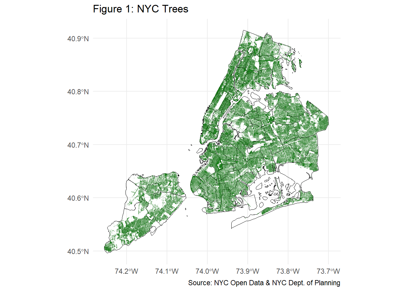
The NYC trees were first mapped by creating a ggplot2 map that superimposes trees as points over the council districts of NYC. Two layers were used to have different spatial elements, one with the council district boundaries and another with points representing each tree.

The district boundary lines were also simplified beforehand for plotting purposes because NYC District shape files are very high resolution and can be somewhat slow to plot.

# Simplification
nyc_council_simplified <- nyc_council |>
  mutate(
    geometry = st_simplify(geometry, dTolerance = 20)
  )

ggplot() +
  # Council district boundaries layer (POLYGON)
  geom_sf(
    data = nyc_council_simplified,
    fill = NA,
    color = "black",
    linewidth = 0.3
  ) +
  # Tree points layer (POINT)
  geom_sf(
    data = trees,
    color = "darkgreen",
    alpha = 0.02,
    size = 0.0005
  ) +
  coord_sf() +
  theme_minimal() +
  labs(
    title    = "Figure 1: NYC Trees",
    caption  = "Source: NYC Open Data & NYC Dept. of Planning"
  )

Improved Tree Map Visualization

The map of all trees is a bit too dense to be truly legible. The following is an interactive visualization to improve legibility.

if (!require("leaflet")) install.packages("leaflet")
library(leaflet)

set.seed(123)

# Sample trees just for performance
trees_sample <- trees |>
  slice_sample(n = 20000) 

leaflet(options = leafletOptions(preferCanvas = TRUE)) |>
  addProviderTiles("CartoDB.Positron") |>
  
  # Title (centered)
  addControl(
    html = "<h3 style='text-align:center; margin:4px;'>Figure 2: Interactive Map for NYC Tree Locations</h3>",
    position = "topleft") |>

  # Council district boundaries
  addPolygons(
    data = nyc_council_simplified,
    color = "black",
    weight = 1,
    fillColor = "grey92",
    fillOpacity = 0.4
  ) |>
  
  # Tree locations as simple points
  addCircleMarkers(
    data = trees_sample,
    radius = 2,
    color = "#006400",   # dark green
    stroke = FALSE,
    fillOpacity = 0.5
  )

Overview

Exploratory data analysis (EDA) was conducted using the st_join function which implements spatial joins between the Tree Points data and the District boundaries. These were the key findings:

# Spatial join between the datasets
trees_with_district <- st_join(
  trees,
  nyc_council,
  join = st_intersects)

# Count trees by district
trees_by_district <- trees_with_district |>
  st_drop_geometry() |>
  group_by(CounDist) |>
  summarise(n_trees = n()) |>
  arrange(desc(n_trees))

# Which council district has the most trees?
district_most_trees <- trees_by_district |>
  slice_max(n_trees, n = 1)

invisible(district_most_trees)

• Council District 51 has the most trees.

# Summarise trees and area per council district
trees_density <- trees_with_district |>
  st_drop_geometry() |>
  group_by(CounDist, Shape_Area) |>
  summarise(n_trees = n()) |> #
  ungroup() |>
  mutate(
    tree_density = n_trees / Shape_Area
  ) |>
  arrange(desc(tree_density))

# District with the highest tree density
district_highest_density <- trees_density |>
  slice_max(tree_density, n = 1)

invisible(district_highest_density)

• Council District 7 has the highest density of trees.

# Count of total trees and dead trees per district
dead_fraction <- trees_with_district |>
  st_drop_geometry() |>
  group_by(CounDist) |>
  summarise(
    total_trees = n(),
    dead_trees  = sum(tpcondition == "Dead", na.rm = TRUE)
  ) |>
  ungroup() |>
  mutate(
    fraction_dead = dead_trees / total_trees
  ) |>
  arrange(desc(fraction_dead))

# District with the highest fraction of dead trees
district_highest_dead_fraction <- dead_fraction |>
  slice_max(fraction_dead, n = 1)

invisible(district_highest_dead_fraction)

• Council District 32 has the highest fraction of dead trees.

# Add Borough based on council district number
trees_with_borough <- trees_with_district |>
  mutate(
    Borough = case_when(
      CounDist >= 1 & CounDist <= 10 ~ "Manhattan",
      CounDist >= 11 & CounDist <= 18 ~ "Bronx",
      CounDist >= 19 & CounDist <= 32 ~ "Queens",
      CounDist >= 33 & CounDist <= 48 ~ "Brooklyn",
      CounDist >= 49 & CounDist <= 51 ~ "Staten Island",
    )
  )

# Keep only trees in Manhattan
manhattan_trees <- trees_with_borough |>
  filter(Borough == "Manhattan")

# Count species in Manhattan
most_common_manhattan_species <- manhattan_trees |>
  st_drop_geometry() |>
  count(genusspecies, sort = TRUE) |>
  slice(1)

invisible(most_common_manhattan_species)

• The most common tree species in Manhattan is Gleditsia triacanthos var. inermis - Thornless honeylocust.

# Helper to create a point with WGS84 CRS
new_st_point <- function(lat, lon, ...) {
  # st_sfc expects x = lon, y = lat
  st_sfc(point = st_point(c(lon, lat))) |>
    st_set_crs("WGS84")
}

# Create a point for Baruch's campus
my_point <- new_st_point(
  lat = 40.7402,
  lon = -73.9834
)

# 2. Compute distance from each tree to Baruch's campus
trees_with_distance <- trees |>
  mutate(
    distance = st_distance(geometry, my_point)
  )

# 3. Find the single closest tree
closest_tree <- trees_with_distance |>
  slice_min(distance, n = 1)

closest_tree_species <- closest_tree |>
  st_drop_geometry() |>
  pull(genusspecies)

invisible(closest_tree_species)

• The tree closest to Baruch’s campus is a Gleditsia triacanthos - Honeylocust.

Proposed NYC Parks Tree Program

The following proposal details a new tree initiative for Council District 26, serving the neighborhoods of Long Island City, Sunnyside, Astoria, and Woodside.

Shade Equity: Increasing Tree Canopy for District 26

Description

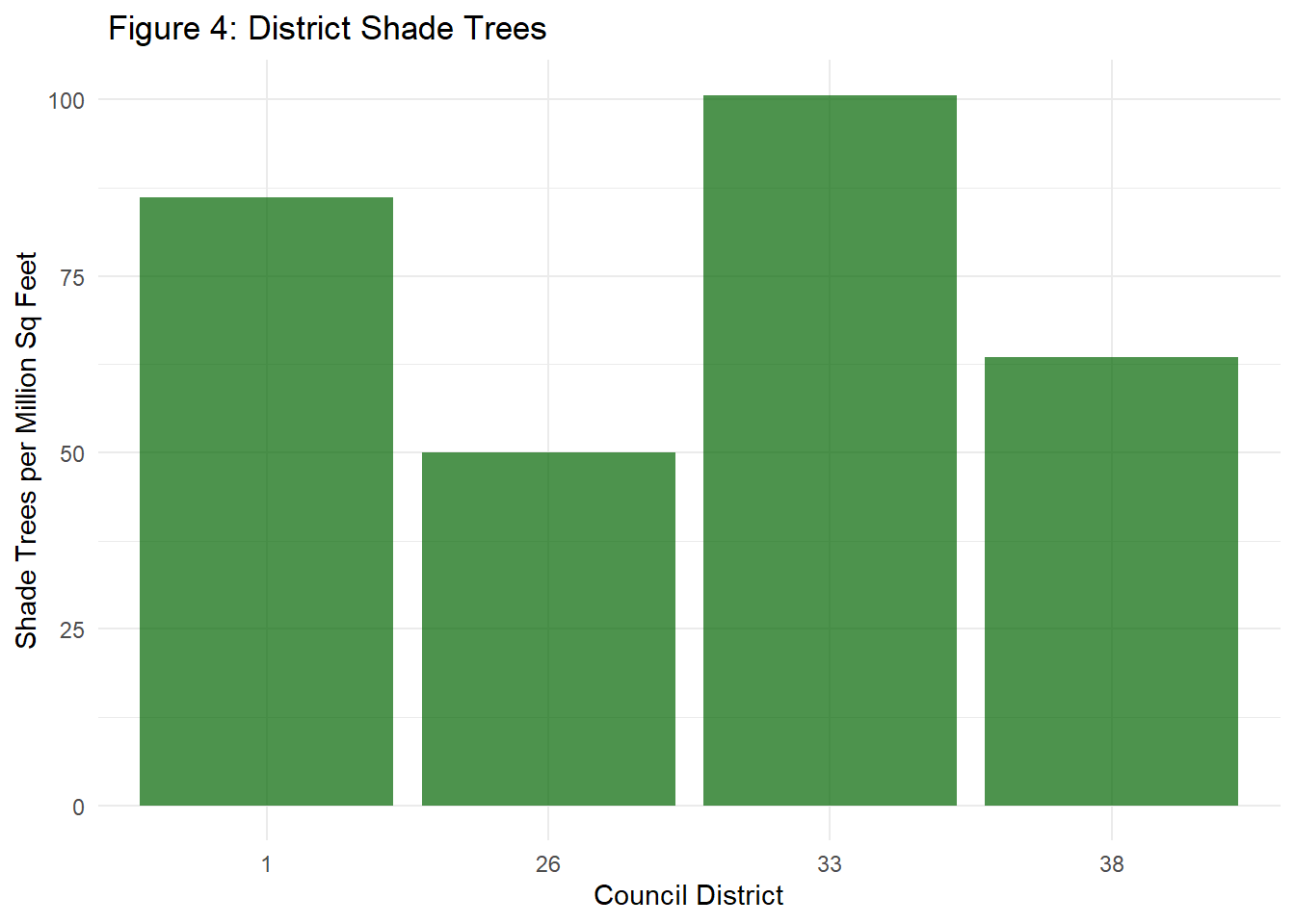
As a resident and council member of District 26, I am proposing a targeted “Shade Equity in District 26” program to increase the amount of tree canopy. District 26 is one of four high-foot-traffic waterfront districts (1, 26, 33, 38). Within this group, it ranks last in shade-producing trees in ratio to its area. District 26 has seen high residential development and heavy pedestrian use, but much of the area remains exposed to full sun. This increases localized heat buildup and makes the district less comfortable for residents to enjoy during hotter seasons.

Scope

# Define a set of broad-canopy "shade" species by species name.
shade_species <- c(
  # Maples
  "Acer nigrum - black maple",
  "Acer platanoides - Norway maple",
  "Acer saccharinum - silver maple",
  "Acer rubrum - red maple",
  "Acer saccharum - sugar maple",

  # Plane / sycamore
  "Platanus x acerifolia - London planetree",
  "Platanus occidentalis - American sycamore",
  "Platanus x acerifolia 'Bloodgood' - 'Bloodgood' London planetree",
  "Platanus x acerfolia 'Exclamation' - 'Exclamation' London planetree",
  "Platanus x acerifolia 'Columbia' - 'Columbia' London planetree",

  # Lindens (Tilia)
  "Tilia cordata - littleleaf linden",
  "Tilia x. europaea - Common linden",
  "Tilia americana - American basswood",
  "Tilia tomentosa - silver linden",
  "Tilia platyphyllos - largeleaf linden",
  "Tilia americana 'Redmond' - 'Redmond' American linden",
  "Tilia americana 'McSentry' - 'McSentry' American linden",

  # Honeylocust
  "Gleditsia triacanthos var. inermis - Thornless honeylocust",
  "Gleditsia triacanthos - Honeylocust",
  "Gleditsia triacanthos var. inermis 'Streetkeeper' - 'Streetkeeper' Thornless honeylocust",
  "Gleditsia triacanthos var. inermis 'Skyline' - 'Skyline' Thornless honeylocust",
  "Gleditsia triacanthos var. inermis 'Imperial' - 'Imperial' Thornless honeylocust",
  "Gleditsia triacanthos var. inermis 'Shademaster' - 'Shademaster' Thornless honeylocust",
  "Gleditsia triacanthos var. inermis 'Northern Acclaim' - 'Northern Acclaim' Thornless honeylocust",

  # Oaks (Quercus)
  "Quercus palustris - pin oak",
  "Quercus phellos - willow oak",
  "Quercus rubra - northern red oak",
  "Quercus alba - white oak",
  "Quercus bicolor - swamp white oak",
  "Quercus x sargentii - Sargent oak",
  "Quercus velutina - black oak",
  "Quercus robur - English oak",
  "Quercus acutissima - sawtooth oak",
  "Quercus macrocarpa - bur oak",
  "Quercus muehlenbergii - chinkapin oak",
  "Quercus lyrata - overcup oak",
  "Quercus coccinea - scarlet oak",
  "Quercus stellata - post oak",
  "Quercus virginiana - live oak",
  "Quercus cerris - European turkey oak",
  "Quercus shumardii - Shumard's oak",
  "Quercus texana - Nuttall oak",
  "Quercus nuttallii - Nuttall oak",
  "Quercus nigra - water oak",

  # Elms
  "Ulmus americana - American elm",
  "Ulmus parvifolia - Chinese elm",
  "Ulmus 'Patriot' - 'Patriot' Elm",
  "Ulmus 'Frontier' - 'Frontier' Elm",
  "Ulmus americana 'Valley Forge' - 'Valley Forge' American Elm",
  "Ulmus americana 'Princeton' - 'Princeton' American elm",
  "Ulmus propinqua 'Emerald Sunshine' - 'Emerald Sunshine' Elm",
  "Ulmus 'New Harmony' - 'New Harmony' Elm",

  # Sweetgum, tuliptree, coffeetree, beech, hackberry, blackgum
  "Liquidambar styraciflua - sweetgum",
  "Liquidambar styraciflua 'Moraine' - 'Moraine' Sweetgum",
  "Liquidambar styraciflua 'Cherokee' - 'Cherokee' Sweetgum",
  "Liquidambar styraciflua 'Grandmaster' - 'Grandmaster' Sweetgum",
  "Liriodendron tulipifera - tuliptree",
  "Liriodendron tulipifera 'Arnold' - 'Arnold' Tulip poplar",
  "Liriodendron tulipifera 'Emerald City' - 'Emerald City' Tulip poplar",
  "Gymnocladus dioicus - Kentucky coffeetree",
  "Gymnocladus dioicus 'Espresso' - 'Espresso' Kentucky coffee tree",
  "Gymnocladus dioicus 'Prairie Titan' - 'Prairie Titan' Kentucky coffee tree",
  "Fagus grandifolia - American beech",
  "Fagus sylvatica - European beech",
  "Celtis occidentalis - common hackberry",
  "Celtis laevigata - sugarberry",
  "Nyssa sylvatica - blackgum",
  "Nyssa sylvatica 'Tupelo Tower' - 'Tupelo Tower' Black gum",
  "Nyssa sylvatica 'Red Rage' - 'Red Rage' Black gum",
  "Nyssa sylvatica 'Wildfire' - 'Wildfire' Black gum"
)

# Filter to District 26 and flag shade trees
district26_trees <- trees_with_borough |>
  filter(CounDist == 26)

district26_shade_summary <- district26_trees |>
  mutate(
    is_shade = genusspecies %in% shade_species
  ) |>
  summarise(
    total_trees    = n(),
    shade_trees    = sum(is_shade, na.rm = TRUE)
  ) |>
  mutate(
    shade_target_20pct = round(shade_trees * 0.20)
  )

invisible(district26_shade_summary)

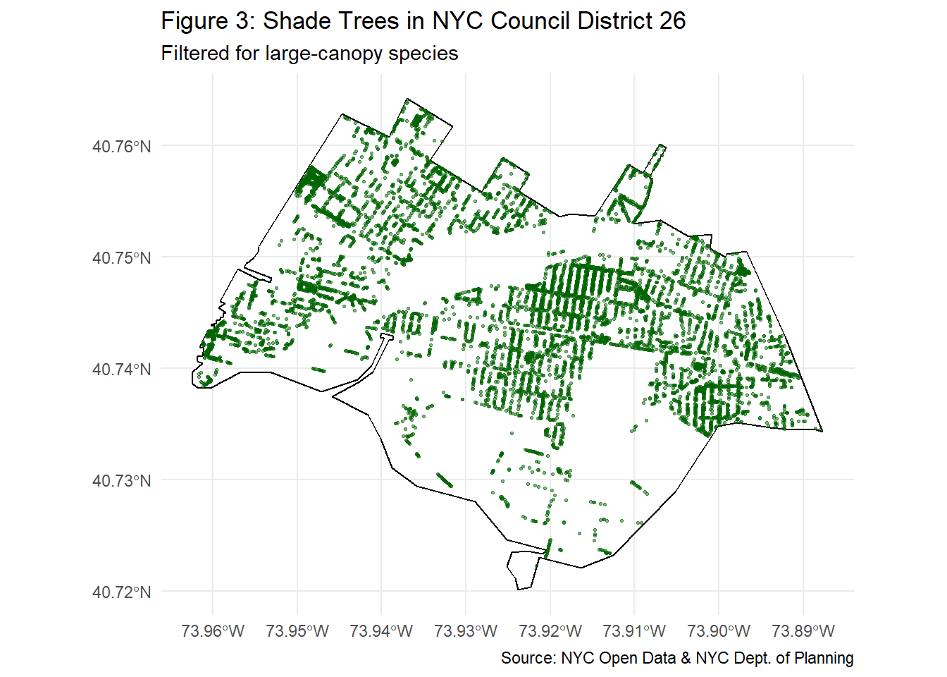
Prior to analysis, a set of broad-canopy “shade” tree species (including maples, plane trees, lindens, oaks, elms, and other large-canopy species) was defined and used to identify shade trees.

# Visualization of shade trees in District 26
district26_shade_trees <- district26_trees |>
  mutate(
    is_shade = genusspecies %in% shade_species
  ) |>
  filter(is_shade)

# District 26 area only
district26_boundary <- nyc_council_simplified |>
  filter(CounDist == 26)

# Plot the trees
ggplot() +
  # District 26 boundary (polygon)
  geom_sf(
    data = district26_boundary,
    fill = NA,
    color = "black",
    linewidth = 0.4
  ) +
  # Shade trees in District 26 (points)
  geom_sf(
    data = district26_shade_trees,
    color = "darkgreen",
    alpha = 0.5,
    size = 0.5
  ) +
  coord_sf() +
  theme_minimal() +
  labs(
    title = "Figure 3: Shade Trees in NYC Council District 26",
    subtitle = "Filtered for large-canopy species",
    caption = "Source: NYC Open Data & NYC Dept. of Planning"
  )

• District 26 currently has 8412 shade trees. Add 20% more, or 1682 new shade trees.

district26_stumps <- trees_with_borough |>
  st_drop_geometry() |>
  filter(CounDist == 26, tpstructure == "Stump") |>
  summarise(
    n_stumps = n()
  )

invisible(district26_stumps)

• Replace the 432 stumps in District 26 with new plantings.

• The altogether addition of 2114 new trees (additional shade trees + replacement of stumps) would increase the total tree count of 15380 trees by ~14%.

• Prioritize broad-canopy species (London plane, red maple, or other large-crown species) to maximize shade per planting location.

Why District 26?

District 26 was compared to three other similarly dense districts with significant waterfront access and heavy foot traffic: District 1 (Lower Manhattan), District 33 (DUMBO/Brooklyn Heights/Williamsburg/Greenpoint), and District 38 (Red Hook/Sunset Park).

# Comparison of shade trees between district 1, 26, 33, 38
shade_by_district <- trees_with_borough |>
  mutate(
    is_shade = genusspecies %in% shade_species
  ) |>
  st_drop_geometry() |>
  group_by(CounDist) |>
  summarise(
    total_trees = n(),
    shade_trees = sum(is_shade, na.rm = TRUE)
  ) |>
  ungroup()

# Area for each district from nyc_council
district_area <- nyc_council |>
  st_drop_geometry() |>
  select(CounDist, Shape_Area)

# Join counts with area and compute shade-tree density
shade_density <- shade_by_district |>
  left_join(district_area, by = "CounDist") |>
  mutate(
    shade_trees_per_million = shade_trees / Shape_Area * 1e6
  )

# Filter districts
shade_density_focus <- shade_density |>
  filter(CounDist %in% c(1, 26, 33, 38)) |>
  arrange(CounDist)

# Bar chart comparing shade-tree density
ggplot(shade_density_focus, aes(
  x = factor(CounDist),
  y = shade_trees_per_million
)) +
  geom_col(fill = "darkgreen", alpha = 0.7) +
  theme_minimal() +
  labs(
    title = " Figure 4: District Shade Trees",
    x = "Council District",
    y = "Shade Trees per Million Sq Feet"
  )

District 26 has the lowest density of shade trees among the comparison districts, only about 50 shade trees per million square feet, which is below Districts 1, 33, and 38.

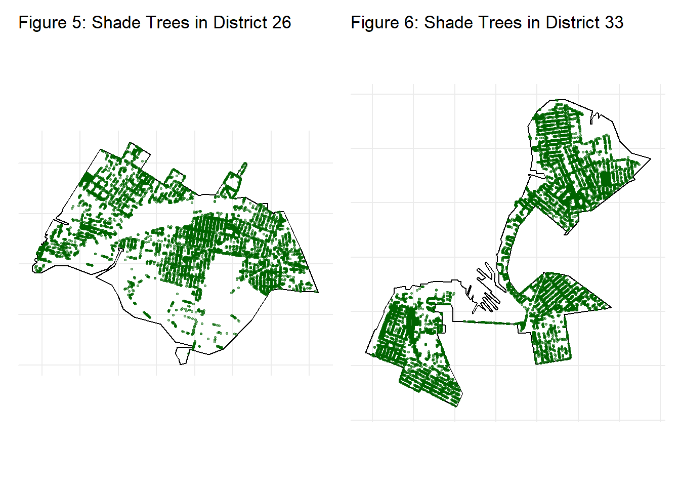
The following visualization illustrates the contrast in shade tree coverage between Districts 26 and 33, neighboring areas that differ significantly in their shade-tree-to-area ratios.

# Trees in District 33
district33_trees <- trees_with_borough |>
  filter(CounDist == 33)

# Shade trees in District 33
district33_shade_trees <- district33_trees |>
  mutate(
    is_shade = genusspecies %in% shade_species
  ) |>
  filter(is_shade)

# District 33 area only
district33_boundary <- nyc_council_simplified |>
  filter(CounDist == 33)

library(patchwork)

# District 26 shade map
p26 <- ggplot() +
  geom_sf(
    data = district26_boundary,
    fill = NA,
    color = "black",
    linewidth = 0.4
  ) +
  geom_sf(
    data = district26_shade_trees,
    color = "darkgreen",
    alpha = 0.5,
    size = 0.5
  ) +
  coord_sf() +
  theme_minimal() +
  theme(
    axis.text  = element_blank(),
    axis.ticks = element_blank(),
    axis.title = element_blank()
  ) +
  labs(
    title = "Figure 5: Shade Trees in District 26",
  )

# District 33 shade map
p33 <- ggplot() +
  geom_sf(
    data = district33_boundary,
    fill = NA,
    color = "black",
    linewidth = 0.4
  ) +
  geom_sf(
    data = district33_shade_trees,
    color = "darkgreen",
    alpha = 0.5,
    size = 0.5
  ) +
  coord_sf() +
  theme_minimal() +
  theme(
    axis.text  = element_blank(),
    axis.ticks = element_blank(),
    axis.title = element_blank()
  ) +
  labs(
    title = "Figure 6: Shade Trees in District 33",
  )

p26 + p33 + plot_layout(widths = c(1, 1))

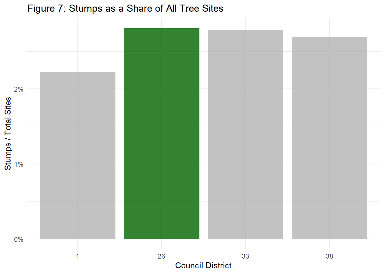
District 26 also has the highest ratio of stumps to total tree sites. In direct comparison, it has significantly higher ratio of stumps to total tree sites than District 1 and slightly higher than District 33 and 38, indicating unrealized planting opportunities.

# Computes stump ratio per district
stumps_by_district <- trees_with_borough |>
  st_drop_geometry() |>
  group_by(CounDist) |>
  summarise(
    total_sites = n(),
    n_stumps    = sum(tpstructure == "Stump", na.rm = TRUE)
  ) |>
  ungroup() |>
  mutate(
    stump_fraction = n_stumps / total_sites
  )

# Comparison of districts
stumps_focus <- stumps_by_district |>
  filter(CounDist %in% c(1, 26, 33, 38)) |>
  arrange(CounDist)

# Bar chart
ggplot(
  stumps_focus,
  aes(
    x = factor(CounDist),
    y = stump_fraction,
    fill = CounDist == 26
  )
) + # highlight District 26
  geom_col(alpha = 0.8) +
  scale_fill_manual(
    values = c("TRUE" = "darkgreen", "FALSE" = "grey70"),
    guide  = "none"
  ) +
  scale_y_continuous(labels = scales::percent_format(accuracy = 1)) +
  theme_minimal() +
  labs(
    title    = "Figure 7: Stumps as a Share of All Tree Sites",
    x        = "Council District",
    y        = "Stumps / Total Sites"
  )

Conclusion

In conclusion, District 26 faces a clear shade equity gap compared with other highly populated waterfront districts. Despite significant residential growth, it has the lowest density of shade-producing trees, a higher stump-to-tree ratio, and large stretches of fully exposed pedestrian areas.